We are troubleshooting an issue impacting community login, and it may be intermittently unavailable. Sorry for any inconvenience.
Hello everybody,
I wonder how can I make a function (for torque motors and others) like this:
f(theta) = g(theta) * theta
where
Solved! Go to Solution.
Once we understand "the flywheel inertia mystery", I returned on the main question in a more general overview.
If one have the function g expressed in a closed form [eg: g(x,y)= f(x)*exp(4y-5); f(x)=sin(x) ] you don't have problems. One can insert the expression inside the "function type: user defined" tab.
One has problems when you have the function f(x) not in a closed form, but with a dots graph. You can't multiply a graph for a function.
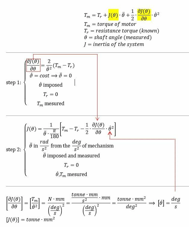
I found a workaround:
I use this method to calculate the J and the J' of the motion equation.
Here are two curve of J(theta): the yellow one comes from the simulation with "my method", the ciano one comes from an algebraic calculus.
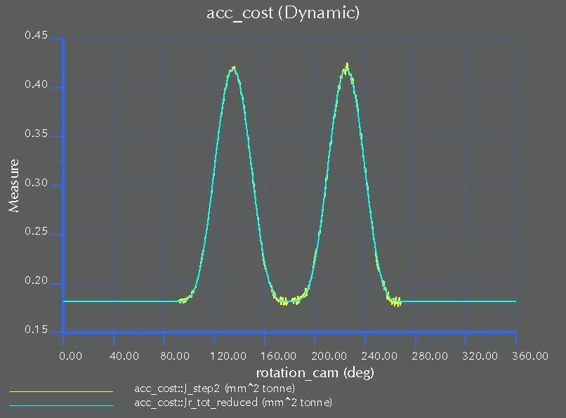
The differences are small and decrease with the number of points growing (the simulation time step).
You must
instead of (g(theta) from external file) * theta
use (g(theta)*theta from external file) = make new external file with the math done.
because no additional math allowed on external file and only one primary variable allowed.
Make new external file using data generated as such.
Example use of external file.
And here is format for .tab file shown using Notepad++ with LINE #s shown
I explain better what I would to to.
I'm studying a mechanical system moved by a brushless motor.
The system is periodic and it can run at a max speed of 140 rpm.
I want to study the initial transitory where the system starts from zero velocity and reaches the max speed.
The brushless motor doesn't have an operation curve, but "a operation field", where the limits are the max speed and the max torque.
I've thought to use the rotating systems equation but I've the inertia and its derivative only like "graph points" and not in closed form like a function.
How can I do?
Great this is good information from you.
I suggest the max torque vs speed as shown. (note x, y axis reversed from your chart)
The operation curve is forced by the controller and so I choose the fastest startup operation.
In simulate use a torque motor with independent variable of speed (not position)
Your rotating systems equation is not for the output torque of the motor, it is for the Load torque the motor must overcome.
Simulate will use mass/geometry/joints to get J(theta) terms and will automatically calculate the inertia based load for you. (I assume you model entire mechanical system and just apply the motor with its proper inertia to it)
You will need to add a constant resistance Tr (bearing drag load) somewhere in your model if you have not already done this.
Note: when simulation reaches operating point (140rpm) then you may need to stop the analysis.
Or make this part of curve slightly sloped like (139.5RPM,Local-Tmax & 140.5RPM,0 ).
This should make it find the constant operating torque Tr.
Also a tip, use the speed units of default (deg/s) for the independent variable. This means your curve must be in terms of deg/s not rpm. You can use a "user defined" measure to convert to RPM but it is best that this is only as final output, not used in equations for motors, forces, etc. (less math during simulation = better)
I inserted the torque-motor datas as you've suggested and, as independent variable, I put the shaft rotation in deg/s (as Creo standard measure).
However I've the trouble the system exceeds the nominal velocity of 140 rpm because the motor velocity is not regulated.
With regard to the initial transient study, all this it's ok; so I tried to study "a normal cycle" that starts at (140 rpm-0 degrees) shaft (velocity-position).
If I study this situation with a servomotor applied to the shaft with a constant velocity, I've seen the system "doesn't feel the shaft inertia": if I apply to the main shaft (where the servo is applied) a fly-wheel, I don't see on the servo's netload any differences beetween the situations with and without fly-wheel.
This is a point that I wonder to the forum community.
Now I want to try with a torque motor...
Inertia is only felt due to accelerations. Since there was constant velocity at the flywheel, the flywheel does nothing. Try ramping the servo velocity slightly and compare with and without the flywheel.
But, I agree, a torque motor shows more what is happening.
If you have CREO5, example files attached.
To make the flywheel changes, just change the density of the large input gear by 10x using the mechanism mass property (change from default)
As expected the flywheel regulates the speed.
Note 839 to 841 deg/s has some real value of slope - otherwise the operating point would be ambiguous.
Watch carefully the extrapolation before and after your defined motor curve.
But, what if we use the motor to apply reverse torque when the speed exceeds our target?
This also compares with and without flywheel.
No problem.
It is possible you want to implement a specific speed control algorithm on the motor torque output. You would need more than just the motor "field" (range of operation)
My speed control algorithm is: if over target, oppose with full negative torque; if under target, oppose with full positive torque. It is not fancy, does not have soft start, PID control, etc.
This chart shows the method, with two example control speeds.
This implements a speed controller.
Note how the motor responds to the speed, working to reach the target.
oops... I just realized I used the wrong login. for some reason my CREO is on one account and Mathcad on this ptc-3239260.
anyway. ptc-3239260 = sweetpeahub
so if you give me kudos I prefer them on sweetpeahub.
Once we understand "the flywheel inertia mystery", I returned on the main question in a more general overview.
If one have the function g expressed in a closed form [eg: g(x,y)= f(x)*exp(4y-5); f(x)=sin(x) ] you don't have problems. One can insert the expression inside the "function type: user defined" tab.
One has problems when you have the function f(x) not in a closed form, but with a dots graph. You can't multiply a graph for a function.
I found a workaround:
I use this method to calculate the J and the J' of the motion equation.
Here are two curve of J(theta): the yellow one comes from the simulation with "my method", the ciano one comes from an algebraic calculus.
The differences are small and decrease with the number of points growing (the simulation time step).