Community Tip - You can subscribe to a forum, label or individual post and receive email notifications when someone posts a new topic or reply. Learn more! X
- Community
- Creo+ and Creo Parametric
- Analysis
- Re: Mechanism Dynamics, Integration Settings, Fram...
- Subscribe to RSS Feed
- Mark Topic as New
- Mark Topic as Read
- Float this Topic for Current User
- Bookmark
- Subscribe
- Mute
- Printer Friendly Page
Mechanism Dynamics, Integration Settings, Frame Rates, and Trace Curves: Observations and Questions
- Mark as New
- Bookmark
- Subscribe
- Mute
- Subscribe to RSS Feed
- Permalink
- Notify Moderator
Mechanism Dynamics, Integration Settings, Frame Rates, and Trace Curves: Observations and Questions
Creo 4, M100
I was playing around with trace curves in a toy mechanism model I created to understand how they behave and I noticed a few things I didn't expect.
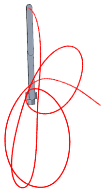
The mechanism I created is a rotating double pendulum - a double pendulum attached to a pivoting center component. The analysis type is dynamic and the only load I have is gravity. There's no friction or damping so no energy loss.
Because the trace curve tool requires a .pbk file and because I understood .pbk files to only be a record of each frame, I wondered how frame rates would affect the trace curve accuracy. So I ran several analyses with different frame rates (1, 10, 100, & 1000, all starting from the same arbitrary snapshot), created trace curves for them, and compared the differences. After 1 second, the difference between 1 FPS & 1000 FPS was less than 1 millimeter. After 2 seconds, the difference was so great that the curves ended on different sides of the assembly.
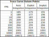
At first, I was surpised to see that even with a frame rate of 1 FPS the trace curve point array had 75 points when I expected only two. The 1000 FPS trace curve had 1001 points like I expected. That made me think that Creo was interpolating between frames in the .pbk so it created as many datum points as necessary to create an accurate trace curve. Pretty neat, I thought - PTC made this tool so it's relatively insensitive to frame rate. But there's no way to accurately interpolate 75 points between just two frames even if you know the positions, velocities and accelerations for them. And why did the 1000 FPS run have the same number of datum points as the frame rate plus one? So what is the .pbk file really recording?
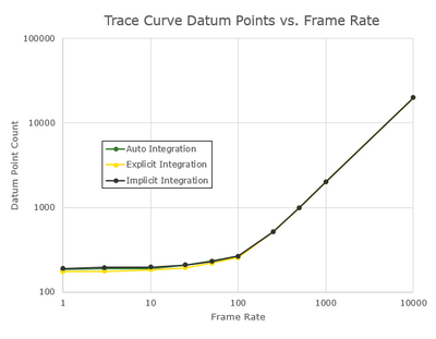
I repeated the above experiment with more FPS settings (1, 3, 10, 25, 50, 100, 250, 500, 1000, 10000) over two seconds and made trace curves for them. When I plotted (log-log) the datum point counts against the frame rates (see the plot below) I saw a curve with two distinct regions: 1) flat at low frame rates with little to no correlation and 2) positive correlation at high frame rates. The curve transitions between 25 FPS & 250 FPS.
The experiments in the last paragraph were done with the default mdo_integration_method setting: "auto". I repeated the experiments with that config option set to "implicit" and "explicit", created trace curves for them, and plotted the datum point counts against the frame rates. See the data and plot below. Although the different integration methods did have an effect on the number of datum points, this was not significant and the three plotted curves (auto, implicit, explicit) were nearly identical.
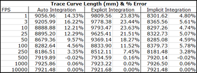
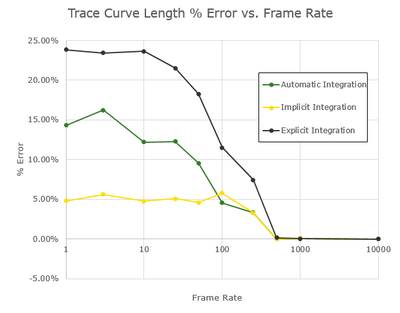
Another metric I used to study this was the lengths of the trace curves. The three 10K FPS trace curves had nearly the same lengths and so I used those values to calculate % error on the other trace curve lengths. When I plotted those % errors I saw significant differences between the three integration methods. See the data and plot below. Explicit integration had the most error at low frame rates and implicit had the least error. It's interesting to note that there was no significant difference after 500 FPS.
I think what's happening here is that at low frame rates the dynamic analysis is automatically lowering (adapting) the analysis time step depending on what the mechanism is doing - during brief moments of high velocity or acceleration for example. The small frame increments with high frames rates are fine enough that Creo never needs to lower the analysis time step below them.
I think the source of my confusion is that the term "frame rate" is misleading. It sounds like the frame rate is just setting how frequently the .pbk file is written, and while that's true, the frame rate also affects the analysis step size. But apparently only at high frame rates and depending on what the mechanism is doing. I understand that my mechanism is a chaotic system in that small changes in initial conditions can wildly affect results, but I'm surprised to learn that "frame rate" can be one of those small changes. In other words, I expected the frame rate to be independent from the analysis time step, but that's not the case.
So, you have the analysis time step which Creo adapts as necessary and you have the frame rate which is the only thing the user has control over. I searched Creo's help file and support.ptc.com, but I didn't find any info on this. I found very little content on frames rates and nothing on the adaptive time stepping.
I should mention that the experiments above were done with a relative mechanism tolerance of 0.001. I may investigate the effect of cranking that up by several orders of magnitude. I also may investigate if kinematic analysis results are affected by frame rates and integration methods as well.
Questions:
What are the rules governing the adaptive time stepping in dynamic analyses?
Is there a way for the user to control the adaptive time step other than through the frame rate?
Is there a way to turn off the adaptive time stepping and have the frame rate be the only control?
Is adaptive time stepping a feature of dynamic analyses only (including static and force balance) or does it work for kinematic analyses as well?
What are the rules governing the number of datum points in trace curves?
What are some examples of situations where one might want to use only implicit integration or only explicit integration?
What are the rules governing when the automatic integration setting switches between implicit and explicit integration?
For the automatic integration setting, will Creo switch between implicit and explicit the middle of an analysis or does it pick one at the beginning of an analysis and use only that?
Is the .pbk file a record or every time step in the analysis or only of each frame?
In summary, these tools are doing things that aren't expected and there's no documentation to explain why. This makes it difficult to trust the results they give. I'd love to hear from PTC on this, but I am prepared to be disappointed.
Solved! Go to Solution.
Accepted Solutions
- Mark as New
- Bookmark
- Subscribe
- Mute
- Subscribe to RSS Feed
- Permalink
- Notify Moderator
Here is an attempt to answer your queries:
What are the rules governing the adaptive time stepping in dynamic analyses?
Rule 1. The Mechanism Engine determines the step size for the integrator based on the local integrator error estimate and user-provided tolerance.
Rule 2. The largest step size that is allowed is the time interval determined by the frame rate. In other words, the smaller of (a) the step size from Rule 1 and (b) the time interval determined by the frame rate, is used for step size.
Is there a way for the user to control the adaptive time step other than through the frame rate?
The only other way is by adjusting the Assembly tolerance (and/or Characteristic Length).
Is there a way to turn off the adaptive time stepping and have the frame rate be the only control?
The only way to do this is to make the frame rate so large (i.e., the frame time interval so small) that it is always smaller than the step size calculated by Rule 1 above.
Is adaptive time stepping a feature of dynamic analyses only (including static and force balance) or does it work for kinematic analyses as well?
It is only for dynamic analysis
What are the rules governing the number of datum points in trace curves?
Number of points is equal to the number or integration steps during analysis run. Since movie file (.pbk) keeps all the information including the intermediate steps data, this allows us to produce trace curves with very good accuracy.
What are some examples of situations where one might want to use only implicit integration or only explicit integration?
If there is a large damping coefficient, use implicit.
If there are many contacts or joint limits, and not too much damping and stiffness, use explicit.
In general, remember that each step of implicit integration is much more computationally expensive than explicit integration, but the advantage of implicit integration is that a larger step size might be possible. If the step size is limited by integration error control, implicit integration is going to be faster. If the step size is not limited by the integration error control but by other factors, e.g., need to keep track of frequently occurring cam contacts, or need to track rapidly oscillating motion, then explicit integration is going to be faster.
What are the rules governing when the automatic integration setting switches between implicit and explicit integration?
An approximation of the largest eigenvalues of the jacobian of the set of differential equations is calculated. Admittedly, this approximation is not always a very good approximation. This is because of the need to calculate this approximation quickly. If the eigenvalues of the jacobian were to be calculated accurately (which is computationally expensive), then one might as well go with implicit integration, and there would be no point in choosing explicit integration. This (not always very good) approximation is used to choose between implicit and explicit integration.
For the automatic integration setting, will Creo switch between implicit and explicit the middle of an analysis or does it pick one at the beginning of an analysis and use only that?
It can switch in the middle. It checks every few steps.
Is the .pbk file a record or every time step in the analysis or only of each frame?
This file keeps data for every time step, including the intermediate steps added during calculations.
- Mark as New
- Bookmark
- Subscribe
- Mute
- Subscribe to RSS Feed
- Permalink
- Notify Moderator
The one certain thing is that frame rate value is which Creo uses to take the values for measures graphs.
I'd like to thank you for the post. It's very clear and useful.
I never done a work like yours (I mean write down a document for a report) but in the past I've done different dynamic analysis and I saw a lot of difference relating the simulation time step. It is true that the program "automatically" increases the time simulation time step, but only (in my opinion) when it feels an high gradient between two (or more) consecutive points.
If your dynamic effect happens mostly among those 2 or 3 points (because of an initial time step too much high) the program may not adapt the time of integration.
I see also another thing related not trace curves, but cams: you should increase not only the simulation accuracy (and the CharacteristicLength) but also the accuracy of the parts involved in the cams' contact.
- Mark as New
- Bookmark
- Subscribe
- Mute
- Subscribe to RSS Feed
- Permalink
- Notify Moderator
I wish Creo gave the user a report of the analysis run itself. When I'm studying a structural problem in Ansys I have control over the initial time step (or number of sub steps), the max and min allowable time steps, if adaptive time stepping is allowed, convergence criteria, and I can look at convergence plots to gauge how well the problem converged. I guess I'm just used to that level of control and insight. Having none of that with MDO makes me feel like I'm flying blind.
I think I'll spend a few hours this weekend rerunning those experiments with different mechanism tolerances. I'm hoping I can come up with some best practices & settings that can be applied to any dynamics problem to maximize accuracy without having to do this kind of iterating every time. I'd like to think that a chaotic system like this is just pushing MDO to its limits and what works here works for any problem, but I'm not sure.
Can you speak more about the characteristic length? Do you typically reduce it from the default value? By how much?
- Mark as New
- Bookmark
- Subscribe
- Mute
- Subscribe to RSS Feed
- Permalink
- Notify Moderator
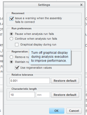
The Characteristic Length is one of two factor which form the Absolute Tolerance (Rel. tol & C.L.).
Normally I set the C.L as the length of the boundary box of the smallest part involved in the simulation.
Usually, for me, it is the cam's roller.
I would suggest you also another thing: turn off the flag over "graphical display during run". Unless your simulation is very simple, that command influences a lot the performance (simulation's duration) without apporting accuracy improvements to the simulation.
- Tags:
- characteristic
- length
- Mark as New
- Bookmark
- Subscribe
- Mute
- Subscribe to RSS Feed
- Permalink
- Notify Moderator
@gfraulini wrote:
Normally I set the C.L as the length of the boundary box of the smallest part involved in the simulation.
Basing the C.L. on the smallest component is surprising, but makes sense. I'll be sure to look at this value in the future. Thanks.
- Mark as New
- Bookmark
- Subscribe
- Mute
- Subscribe to RSS Feed
- Permalink
- Notify Moderator
Here is an attempt to answer your queries:
What are the rules governing the adaptive time stepping in dynamic analyses?
Rule 1. The Mechanism Engine determines the step size for the integrator based on the local integrator error estimate and user-provided tolerance.
Rule 2. The largest step size that is allowed is the time interval determined by the frame rate. In other words, the smaller of (a) the step size from Rule 1 and (b) the time interval determined by the frame rate, is used for step size.
Is there a way for the user to control the adaptive time step other than through the frame rate?
The only other way is by adjusting the Assembly tolerance (and/or Characteristic Length).
Is there a way to turn off the adaptive time stepping and have the frame rate be the only control?
The only way to do this is to make the frame rate so large (i.e., the frame time interval so small) that it is always smaller than the step size calculated by Rule 1 above.
Is adaptive time stepping a feature of dynamic analyses only (including static and force balance) or does it work for kinematic analyses as well?
It is only for dynamic analysis
What are the rules governing the number of datum points in trace curves?
Number of points is equal to the number or integration steps during analysis run. Since movie file (.pbk) keeps all the information including the intermediate steps data, this allows us to produce trace curves with very good accuracy.
What are some examples of situations where one might want to use only implicit integration or only explicit integration?
If there is a large damping coefficient, use implicit.
If there are many contacts or joint limits, and not too much damping and stiffness, use explicit.
In general, remember that each step of implicit integration is much more computationally expensive than explicit integration, but the advantage of implicit integration is that a larger step size might be possible. If the step size is limited by integration error control, implicit integration is going to be faster. If the step size is not limited by the integration error control but by other factors, e.g., need to keep track of frequently occurring cam contacts, or need to track rapidly oscillating motion, then explicit integration is going to be faster.
What are the rules governing when the automatic integration setting switches between implicit and explicit integration?
An approximation of the largest eigenvalues of the jacobian of the set of differential equations is calculated. Admittedly, this approximation is not always a very good approximation. This is because of the need to calculate this approximation quickly. If the eigenvalues of the jacobian were to be calculated accurately (which is computationally expensive), then one might as well go with implicit integration, and there would be no point in choosing explicit integration. This (not always very good) approximation is used to choose between implicit and explicit integration.
For the automatic integration setting, will Creo switch between implicit and explicit the middle of an analysis or does it pick one at the beginning of an analysis and use only that?
It can switch in the middle. It checks every few steps.
Is the .pbk file a record or every time step in the analysis or only of each frame?
This file keeps data for every time step, including the intermediate steps added during calculations.
- Mark as New
- Bookmark
- Subscribe
- Mute
- Subscribe to RSS Feed
- Permalink
- Notify Moderator
Arnaud,
Thank you very much for the excellent answers and the reference document. I wish I could give you a kudos for each question.
That all makes sense to me and jives with what I've seen.
Thanks & regards,
-Andrew
- Mark as New
- Bookmark
- Subscribe
- Mute
- Subscribe to RSS Feed
- Permalink
- Notify Moderator
I thought I'd give this dead horse a few more whacks for good measure. I repeated my frame rate experiments for different mechanism tolerances and characteristic lengths.
First, I looked at the effect of decreasing the characteristic length to match the bounding box size of the smallest component, 170mm. All the previous experiments were done with a characteristic length of ~360mm. I don't know why what value was default as it's smaller than the smallest bounding box of the mechanism.
Changing from 360mm to 170mm while maintaining a mechanism tolerance of 1E-3 had no effect on the number of trace curve datum points or trace curve lengths. See the data below. All measurements were precisely the same for all frame rates I looked at. I'm not sure what conclusions you can draw from this. Either this has something to do with the peculiarities of my model or 360mm was an appropriate value to begin with and and lowering it any further has no effect.
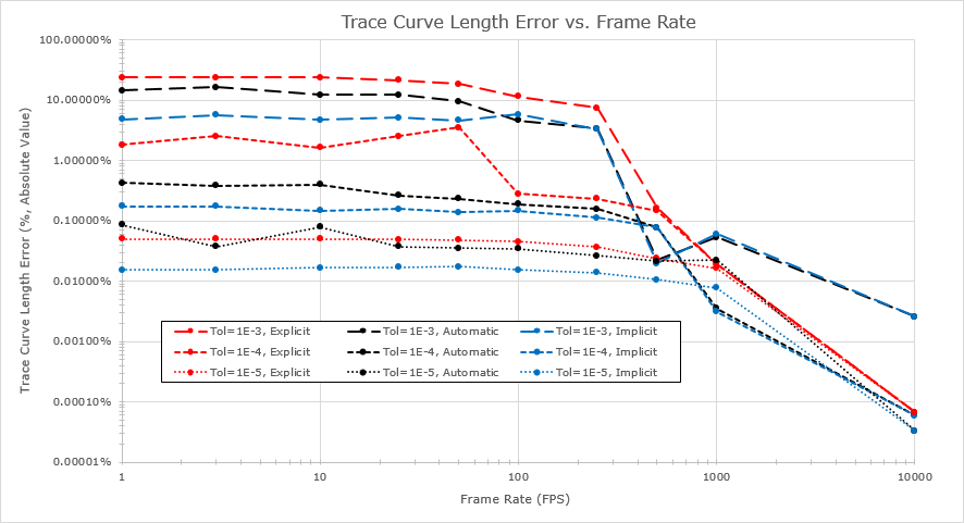
Next, I set the mechanism tolerance to 1E-4 and 1E-5 while maintaining the characteristic length of 170mm. The datum point counts increased at low frame rates and remained unchanged at ultra-high frame rates. This makes sense since the number of datum points equals the number of integration points. At ultra-low frame rates the adaptive time stepping dominates and at ultra-high frame rates the frame rate interval dominates.
Finally, I measured trace curve lengths and calculated errors. I based the error calculations on the average lengths of the three 10k FPS runs with 1E-5 tolerance.
Even at ultra-low frame rates, the precision you get with lower tolerances is better than what you get with high frame rates at lower tolerances. In other words, you get more analytical bang for your computational buck with lower tolerance. I didn't measure solve times for these runs, I wish I knew how, but low frame rate runs with low tolerance did solve quicker than high frame rate runs with higher tolerance.
I'm hesitant to draw generic conclusions from this one model to apply to any dynamics problem, but one thing I think I'll do from now on is to always use a mechanism tolerance of 1E-4 or less.

