Community Tip - When posting, your subject should be specific and summarize your question. Here are some additional tips on asking a great question. X
- Subscribe to RSS Feed
- Mark Topic as New
- Mark Topic as Read
- Float this Topic for Current User
- Bookmark
- Subscribe
- Mute
- Printer Friendly Page
Is there a more efficient way to solve the Colebrook-White Equation?
- Mark as New
- Bookmark
- Subscribe
- Mute
- Subscribe to RSS Feed
- Permalink
- Notify Moderator
Is there a more efficient way to solve the Colebrook-White Equation?
Please see the attached MC Prime 3.0 worksheet (I also included a PDF copy for users of other versions of MC).
Introduction (for those who don't know the Colebrook White Equation)
The empirical Colebrook-White Equation (CW) is the standard way to estimate friction factors for use with the Darcy Equation for determining energy (head) loss in fluid flow. CW has three variables: the relative roughness (k), the Reynolds Number (NR), and the friction factor (f). The relative roughness describes the pipe condition, the Reynolds Number describes the fluid condition, and the friction factor is based on these two. CW is normally solved for f based on input values of k and NR. CW is implicit for f and requires an iterative solution.
Instead of interating CW, it is possible to use the Moody Diagram to find f. The Moody Diagram has NR as the independent varaible and f as the dependent variable. A family of curves, each based on a constant value of k is plotted in the turbulent flow region. Knowing k reduces the problem to just two variables, NR and f.
The Problem
I am working on plotting my own Moody Diagram in Mathcad. I have done this in Excel and CurveExpert Pro, but now I want to do it Mathcad. Also, I am comparing various explicit approximations to CW for accuracy (I have already completed the smooth pipe analysis for k=0). For both tasks, I need an efficient way to solve CW over the ranges of k and NR. For example, I have a data set consisting of 21 values for k and 45 values for NR, which gives me 945 data points for f in 21 cuves (in the attached worksheet, I reduced the data set for NR to 23).
As you can see in the attached worksheet, I was able to solve CW. However, I am looking for a more efficient and more elegant method. I tried various combinations of subscripts, vectorize operations, etc. both inside and outside the solve block, but this is the best I was able to do. Any suggestions would be greatly appreciated.
Solved! Go to Solution.
- Labels:
-
Statistics_Analysis
Accepted Solutions
- Mark as New
- Bookmark
- Subscribe
- Mute
- Subscribe to RSS Feed
- Permalink
- Notify Moderator
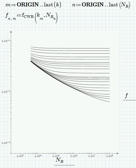
If a 2D matrix is plotted the plot type in Prime 2 had to be set to waterfall plot explicitely to make it work the way we are used from older Mathcad. In Prime 3 waterfallplot is chosen automatically in that case.
- Mark as New
- Bookmark
- Subscribe
- Mute
- Subscribe to RSS Feed
- Permalink
- Notify Moderator
How about the attached? In MC15 format I'm afraid as I don't have Prime 3.
Alan
Edit: Just realised that, if Prime 3 is like Prime 2, the 2D plotting won't be possible using the single friction factor variable in the way that is possible in MC15.
- Mark as New
- Bookmark
- Subscribe
- Mute
- Subscribe to RSS Feed
- Permalink
- Notify Moderator
If a 2D matrix is plotted the plot type in Prime 2 had to be set to waterfall plot explicitely to make it work the way we are used from older Mathcad. In Prime 3 waterfallplot is chosen automatically in that case.
- Mark as New
- Bookmark
- Subscribe
- Mute
- Subscribe to RSS Feed
- Permalink
- Notify Moderator
Thanks, Alan. That was the magic I was looking for. I got closer to the matrix I wanted with the augment command, but that was brute force. Your solution was simple and elegant.
- Mark as New
- Bookmark
- Subscribe
- Mute
- Subscribe to RSS Feed
- Permalink
- Notify Moderator
Here is a bit late pretty much the same as Alan showed done in Prime with your data. MC15 plots just look better, though, and are much easier to format.

- Mark as New
- Bookmark
- Subscribe
- Mute
- Subscribe to RSS Feed
- Permalink
- Notify Moderator
Thanks, Werner. Now to apply this to the bigger worksheet I am working on.
- Mark as New
- Bookmark
- Subscribe
- Mute
- Subscribe to RSS Feed
- Permalink
- Notify Moderator
You are welcome.
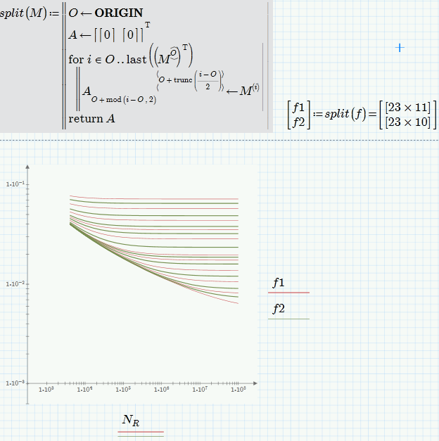
In case you want to retain the alternating colors in your plot, you may consider using a routine to split the matrix f accordingly.

- Mark as New
- Bookmark
- Subscribe
- Mute
- Subscribe to RSS Feed
- Permalink
- Notify Moderator
That is a very clever program. However, for comparison purposes, I am going to be plotting a second data set from an explicit formula that attempts to approximate Colebrook-White, so having one data set in black and the other in red will actually work better for me. Actually, I am comparing 21 explicit formulas to Colebrook-White, so I will end up with 21 plots.


