FFT amplitude resolution and log scale plotting problems

[ptc-3089498]

Hello,

I used the FFT in Mathcad and compared the results to other programs like Igor and Matlab.

In the attached example, I performed the FFT on a sinewave and got the expected peak at my sinewave frequency. This is great, but the the other points close to the fundamental seem quite high in amplitude. I also notice this in other Mathcad FFT plots/examples I see on line. In the other programs I mentioned, the points close to the fundamental have very low magnitude as they should. I think I am doing something wrong and appreciate some comments.

The last plot in my example shows and attempt to plot the FFT with a vertical log scale.As you can see, I get a horizontal line at 1 and the bar graph bars are referenced to that. I would like to get the bar graph lines stating at the "noise floor" of my meaurement and end on the spectral magnitude. Can anyone suggest a way to get the FFT to display the way I would like it to?

Thank you

[Fred_Kohlhepp]

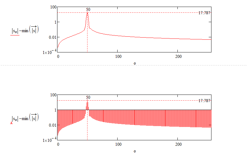
I've subtracted the minimum value (so the graph should start at zero, and plotted a line insted of bars. Any help?

[ptc-3089498]

Hi Fred,

Thank you for your help.

I modified your plot to display bars and got the same result as before; a horizontal line at 1 which serves as the origin for all bars.

You can see this in the images below.

John

[ptc-3089498]

Related to the other problem I am haiving with FFT spurs, I verified that my sinewave has amplitude of 0 at time 0 and time 2047.

[Fred_Kohlhepp]

I suspect that the issue with the bar plot is related to Mathcad trying to draw from zero to the data point on a log plot; it can't find zero, so it finds e^0 =1.

The issue with "spurs" is tied up in resolution (number of points in your vectot) and sampling frequency. See attached.

[ptc-3089498]

Hi Bill,

Thank you once again for your help.

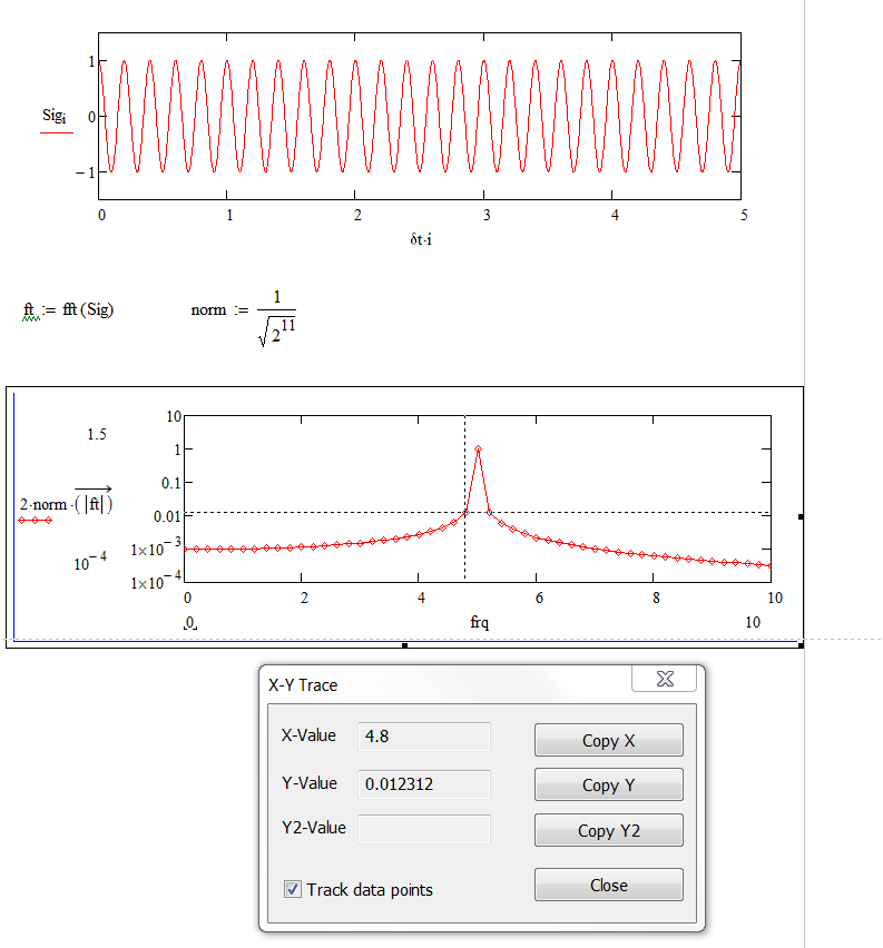
I modified you file to use log scaling on the y axis. Your log scaled plot has the same issue as mine. The 4.8 Hz spectral line has a magnitude of 0.012 and it should be very close to zero. I have yet to see an example of a Mathcad FFT with low spurious.

John

[Fred_Kohlhepp]

If you do this with another program (Matlab? Igor?) what does the same point show?

[ptc-3089498]

Hi Fred,

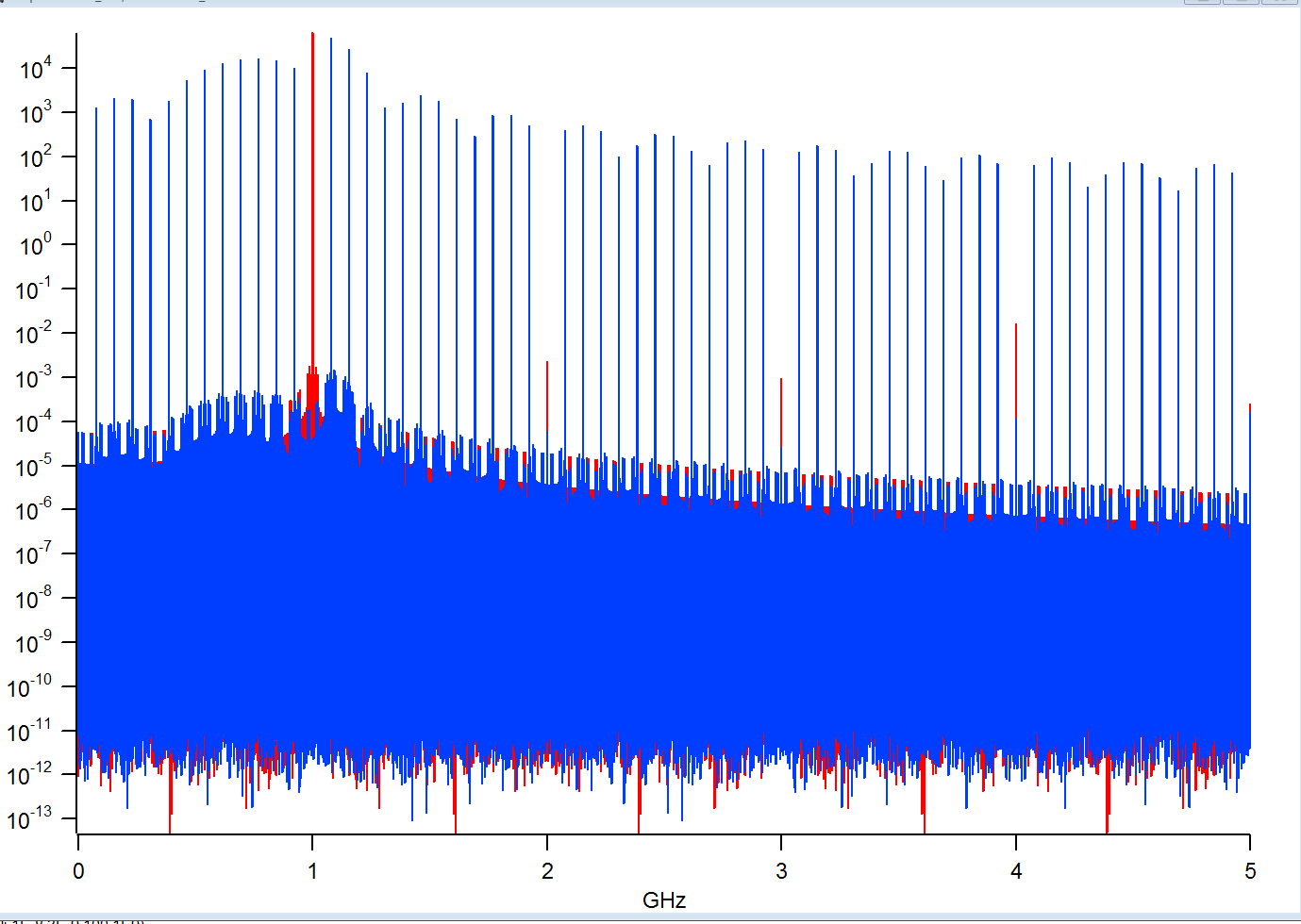
Here is an example of Igor's FFT output. Nothing special was done to get this plot. You can see that there are seven orders of magnitude difference between the signals that should be there and those that shouldn't. I am going to try a Blackman window on my signal before FFT to see if that helps Mathcad get the right answer.

John

[Fred_Kohlhepp]

I'm not sur what I'm looking at; but it's not my example!

If you put my exact example into Igor, what does it give you?

The fft math is the same--I'd expect the same answer from Igor, Matlab or Mathcad.

[ptc-3089498]

Hi Fred,

I am a bit short of time now. I will try to get to doing your exact example in Igor. My point in presenting the plot I did was to show that Igor's dynamic range is HUGE compared to Mathcad when it comes to FFT results.

As I mentioned earlier, I seearched quite a bit on line and never saw a Mathcad FFT plotted on a log scale that didn't have the same problems we are discussing. All the Mathcad FFT plots I saw that look pretty were done with a linear magnitude scale.

As far as plotting bar graphs on a log scale, I wonder if what I see is a Mathcad bug?

[ptc-3089498]

So here is the result with a Blackman window. It looks better in that I now have a reasonable noise floor. Of course the main spectral lobe is wider, but that the window's fault.

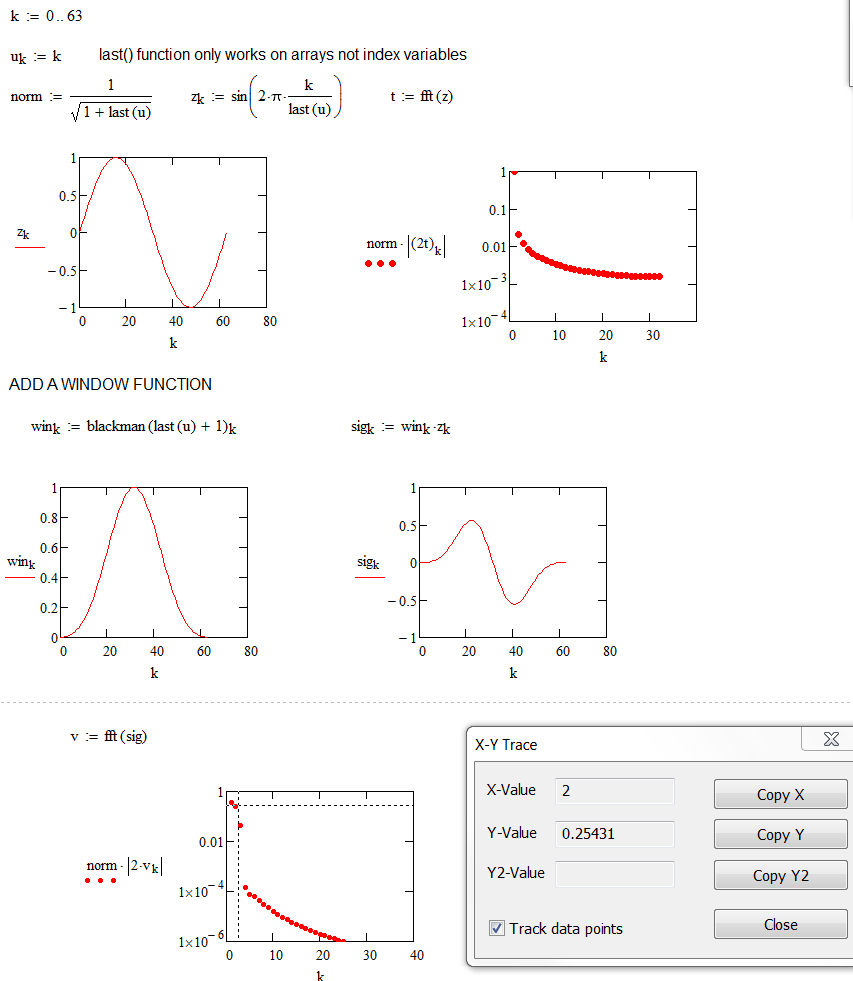
So Can Mathcad yield a decent FFT? Maybe yes maybe no, I will dig into this further but I may just avoid Mathcad for FFTs. I'll post a Matlab example next week when I have more time.

[ptc-3089498]

Here is the same 5Hz 1V sinewave plotted with Igor. The blue trace is the FFT computed with single precision, and the red one was computed with double precision. No windowing was used and the results are what one would expect from a good FFT. With single precision, the points on either side of the 5 Hz peak are 7 orders of magnitude down. With double precision, the points on either side are 15 orders of magnitude down.

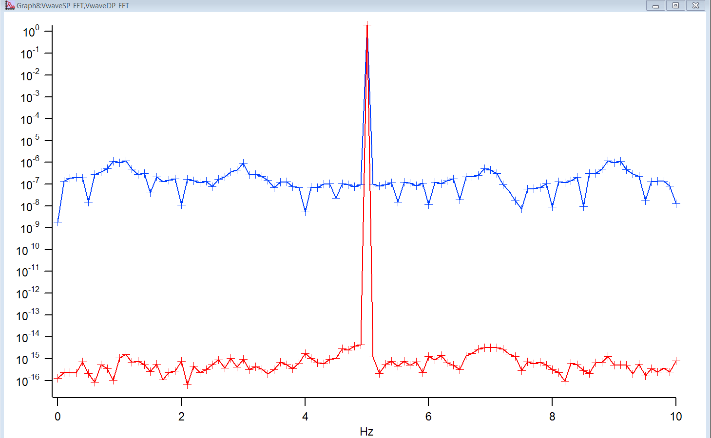
Has anyone been able to get this good a result with Mathcad?

[Fred_Kohlhepp]

Best I can do; sample size is choking memory. Maybe Prime?

Why all the irregularity in your traces?

[ptc-3089498]

Hi Fred,

Thanks for your reply.

>>Best I can do; sample size is choking memory. Maybe Prime?

Are you refering to Mathcad or Igor?

Not sure what you mean here, can you explain?

>>Why all the irregularity in your traces?

I assume you are refering to the Igor plot I showed. If you are refering to something else please let me know.

The irregularity you see is called noise. It results from reaching the limits determined by the precision of the numbers used in the FFT computation. It is actually quite healthy to see this in an FFT because it means that you have maximum possible signal to noise ratio determined by the precision of your math not by something funky going on in the FFT algorithm. From the plots given in previous messages, Igor has as a noise floor at 10^-7 for single precision and 10^-15 for double precision FFT's. Mathcad has spurs as high as 10^-2. That is a huge performance deficit for Mathcad; 5 to 13 orders of magnitude in fact!

If anyone has any information on how to get high quality wide dynamic range FFT plots with Mathcad, I am very interested to learn your method.

[Fred_Kohlhepp]

John Pease wrote:

Are you refering to Mathcad or Igor?

Not sure what you mean here, can you explain?

Mathcad Prime 2.0 can run two different levels (16 bit and 32 bit?). My poor computer (at work) is running Mathcad 14.0, and chokes if I chose a larger sample size than 2^23. (The larger the sample, the better the resolution, the lower the "noise floor.") A better computer can take a larger sample and lower the "noise floor" even more.

John Pease wrote:

I assume you are refering to the Igor plot I showed. If you are refering to something else please let me know.

The irregularity you see is called noise. It results from reaching the limits determined by the precision of the numbers used in the FFT computation. It is actually quite healthy to see this in an FFT because it means that you have maximum possible signal to noise ratio determined by the precision of your math not by something funky going on in the FFT algorithm. From the plots given in previous messages, Igor has as a noise floor at 10^-7 for single precision and 10^-15 for double precision FFT's. Mathcad has spurs as high as 10^-2. That is a huge performance deficit for Mathcad; 5 to 13 orders of magnitude in fact!

If anyone has any information on how to get high quality wide dynamic range FFT plots with Mathcad, I am very interested to learn your method.

Bear with me, what noise? This example was (mathematically) a perfect 5 Hz sine wave. So theoretically there is no noise. Digital bit flutter?

We've got a basic disconnect somewhere.

[ptc-3089498]

Hi Fred,

Thank you for your reply.

So with a lot more samples you can get the noise floor down. What is the best signal to noise ratio (SNR) you can achieve with your Mathcad example?

So far, without windowing I can only achieve achieve about 100:1 SNR because of spurs.

A mathematically perfect sinewave with a mathematically perfectly calculated FFT will have a single line in the spectrum at the fundamental frequency and zero everwhere else. When you use less than perfect math you get noise. But since I am just an engineer, I feel quite comfortable ignoring it when it is 7 or 15 orders of magnitude down from my signal. However as an engineer, I do care about unexplained sprurs which are only two orders of magnitude down.

The real goal here is to try to learn why these large spurs occur in Mathcad and what can be done to eliminate them.. My Igor example was given to show what is possible, not to generate a discussion about why Igor has noise problems 7-15 orders of magnitude below my signal.

For what I do the noise plotted in Igor can be neglected, but maybe for what you do it is a concern. "Digital Signal Processing" by Oppenheim and Shafer has a very good chapter on the effects of finite register length in DSP computations. You might be interested in what they have to say about the subject.

Has anyone come up with a way to get Mathcad FFTs without these large spurs?

[PhilipOakley]

The maths of the fast fourier transform is obviously digital, but what that means in reality isn't always fully appreciated. In this case what it means is that the only frequencies that are posssible are exactly those at the multiples of 1/(T). i.e. once cycle per sample vector length, two cycles per sample vector length, three cycles, 4 cycles, etc.

So if you have a signal which is not quite at one of those spot frequencies, then the maths will split it into lots of bits at the allowed frequencies. Obviously it will have its main component at the nearest multiple, and there will be a roll-off either side (usually shaped in a 'sin(x)/x' profile). This may be part of your side spur issue.

There are also a few issues about how the noise floor varies with the sample rate which can depend on the external filtering, the sampling aperture time, etc., but that's a more than a short note 😉

[RichardJ]

Has anyone been able to get this good a result with Mathcad?

See my other post.

I don't know what you have programmed in Igor, but I will make an observation that might lead you to where the difference is:

With ORIGIN=0, rows(u)=last(u)+1

With ORIGIN=1, rows(u)=last(u)

[MichaelH]

Your two issues in the original worksheet are

1) the spectrum near the peak appears spread (what you call "spurs") and

2) the amplitude far away from the peak ("noise floor") should be significantly lower by orders of magnitude.

The issues are due to two sources:

1) the spreading near the peak is caused by your "time varying phase shift" term. This term basically adds spectral energy at frequencies around the peak frequency. It is real and not a bug with the FFT. If you create another function with the "time varying phase shift" term removed, you will see the spreading decreases significantly.

2) the high "noise floor" is due to the period (frequency) of the function being slightly off. The 2048th point should be 0, yet you have it as the 2047th. You can see this by noting that when the function crosses the X-axis, the Y-value is not that close to 0 in many cases. If you change your n value to 2048 and modify your o index to 0...n-1, you'll see that the function crossing valuess are much closer to the X-axis, and the frequency of the theoretical peak is closer to being an integer multiple of your X-axis index. If you do this for the case I described in #1, you'll see for the function with the "time varying phase shift" term removed that the noise floor goes to 10^-14 and the peak appears as a single point, which is what one would expect.

We often get people coming in here thinking that somehow Mathcad is a defective or buggy product compared to more well known packages like Matlab or Mathematica. Although some bugs in Mathcad have been spotted and reported here, the overwhelming source for issues is the user making a simple error (like being off by 1 in counting) or misunderstanding how a function works (usually caused by not reading the extensive HELP files), but sometimes the issues are not easy to spot and it's good that there is a forum here where people who pay the rent using Mathcad can give their two cents.

[PhilipOakley]

if you want you want to avoid the awkward Log(0)=1 baseline for the bar chart style of plot, but still want uprights then

(a) you can use the stem plot because it uses the same baseline, but

(b) you can use the Error bar style of plot (you need to see the work example in the tutorial).

I tried it by firstly detecting the noise floor by doing a vectorised min of the amplitude, and recreating a noise floor vector. It is then used as the lower limit of the errror bar graph. This gives you the plot you desire.

I'd add the file but the web editor is rubbish.

[PhilipOakley]

See if this adds the file

[RichardJ]

That is not a perfect sine wave, because what you have is not exactly one period. The first point is duplicated at the end, and it should not be. You can easily see this from two things:

1) The FFT does not produce a purely imaginary result, which it should do

2) When you stack the "periods" you end up with pairs of zeros where they join.

Computer roundoff is certainly something to watch for, but when you get "roundoff errors" as big as the errors you are seeing, they are not roundoff errors. It could only be a bug in the FFT or an error in the worksheet.