A friendly hello,
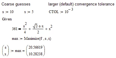
In the attached calculation it is easy to see from the angle sums (they must be 180°) that coarser starting values produce less precise results. Are there settings in MC14 that achieve good calculation results even with coarser starting values? Currently, the iteration can only be made successful in the sense of a fixed point equation with almost exact starting values.
Solved! Go to Solution.
Its not always a good idea to set the convergence tolerance CTOL to a value too small. It may result (as in your case) that no solutions are found with bad guess values.
Setting CTOL to its default value 10^-3 gives us results even with coarse guesses, as you can see.
Of course numerical inaccuracies are inevitable, especially for some bad conditioned approaches.
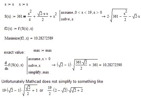
In your case its sure better to solve the constraint and insert it into the objective function.
Then "Maximize" sure gives a numerical result much closer to the exact one which you also can get using the zero of the derivative.
You have just one equation but want to maximize the area by modifying two variables (x and s). Irritating that you use x for the name name the y-coordinate of point A 😉 But then, x is also the x-coordinate of D ...
You try to maximize a function with two independent (which IMHO is wrong, see below) variables x and s. Chances are that the corresponding surface has a lot of different local maximas and so it may strongly depend on the guess values which one you get.
IMHO the length s=BC cannot be chosen independently from x as s depends on x. Look at the right angled triangle OCA with the cathets x and x+s/2 and the hypotenuse 19 and apply Pythagoras.
So we get:
BTW, the original task of @ttokoro (area given with 60) can now also be solved that way:
BTW you may also change the task and ask for the area of ABC where the length AB is minimal 😉 This modified task has the same solution because when AB is minimal, the area ABC is maximal.
Here is a little animation showing area ABC, length AB and length BC as well as the geometry depending on the value chosen for x=OA=OD.
Mathcad 15 file attached.
Thank you for the detailed explanations and especially for the graphical representations. But I'm afraid that I didn't formulate my question clearly enough and that there is therefore a misunderstanding. Regardless of the geometric background (the problem is quite easy to solve and is currently not the topic), my concern is the following:
Given is a function in two variables that has to be maximized under a secondary condition. The MC calculus requires starting values for the solution in the solution block. If these are chosen too far away from the solution, as in the present case, a very inaccurate numerical solution is created. And this is surprising when, after solving the constraint for x and inserting it into the function f(s,x) to be maximized as a function h(s) (see attached file), you get a curve with an obviously easily recognizable maximum and a larger monotonic environment (respectively left and right). The gradient method should then also tolerate coarser starting values when approximating on both sides in order to lead to a numerically precise solution.
I previously had similar problems in more complicated optimization tasks in multiple variables with multiple constraints. These can usually be solved by adjusting the TOL and CTOL.
Its not always a good idea to set the convergence tolerance CTOL to a value too small. It may result (as in your case) that no solutions are found with bad guess values.
Setting CTOL to its default value 10^-3 gives us results even with coarse guesses, as you can see.
Of course numerical inaccuracies are inevitable, especially for some bad conditioned approaches.
In your case its sure better to solve the constraint and insert it into the objective function.
Then "Maximize" sure gives a numerical result much closer to the exact one which you also can get using the zero of the derivative.
Hello @Werner_E ,
Since I don't have M15, can you please expand on how the animation is done?. Is that a M15 feature? What is the technique to make the animation?
Yes, animations are a Mathcad feature. As far as I remember some kind of animations is planned for future (?) Prime versions.
Animations in Mathcad are quite simple. There is a variable FRAME which, when you create an animation, runs from 0 to any number you want (up to 999). This also means that animations are limited to a max of 1000 frames.
Its up to you to depend all variables which you would like to animate on that single FRAME variable. Then you select an area in your sheet which you want to see in the animation and let Mathcad do. It will create an animation which you can save in an avi container using a very old, inefficient codec which supports only a limited number of colors, so you may see different colors compared to what you see in your Mathcad sheet.
Because I feel that handling avi and other videos in this forum is quite clumsy and uncomfortable, I used an online-converted to turn the avi into an animated GIF and inserted this in my posting.
Find attached the original avi file created by Mathcad (it has the advantage that you can watch it frame by frame using an appropriate movie viewer. The animation was created using 301 frames in total.
Here is the complete setup in Mathcad. only x is made dependent on FRAME. The if function was necessary because I wanted a back and forth movement so that the animation starts and ends with x=0.
BTW, I mis-read the explanation text in the sheet of @AlfredFlaßhaar and supposed that he used the name "x" the y-coordinate AO of point A. But he rather used the name "x" for the length AD. So 'my' x and his differ by the factor sqrt 2.