cancel
Showing results for 
Search instead for 
Did you mean: 
cancel
Showing results for 
Search instead for 
Did you mean: 

Community Tip - Did you know you can set a signature that will be added to all your posts? Set it here! X

Matlab Code to Mathcad (15) - FE

Cornel
19-Tanzanite

Matlab Code to Mathcad (15) - FE

Hello,

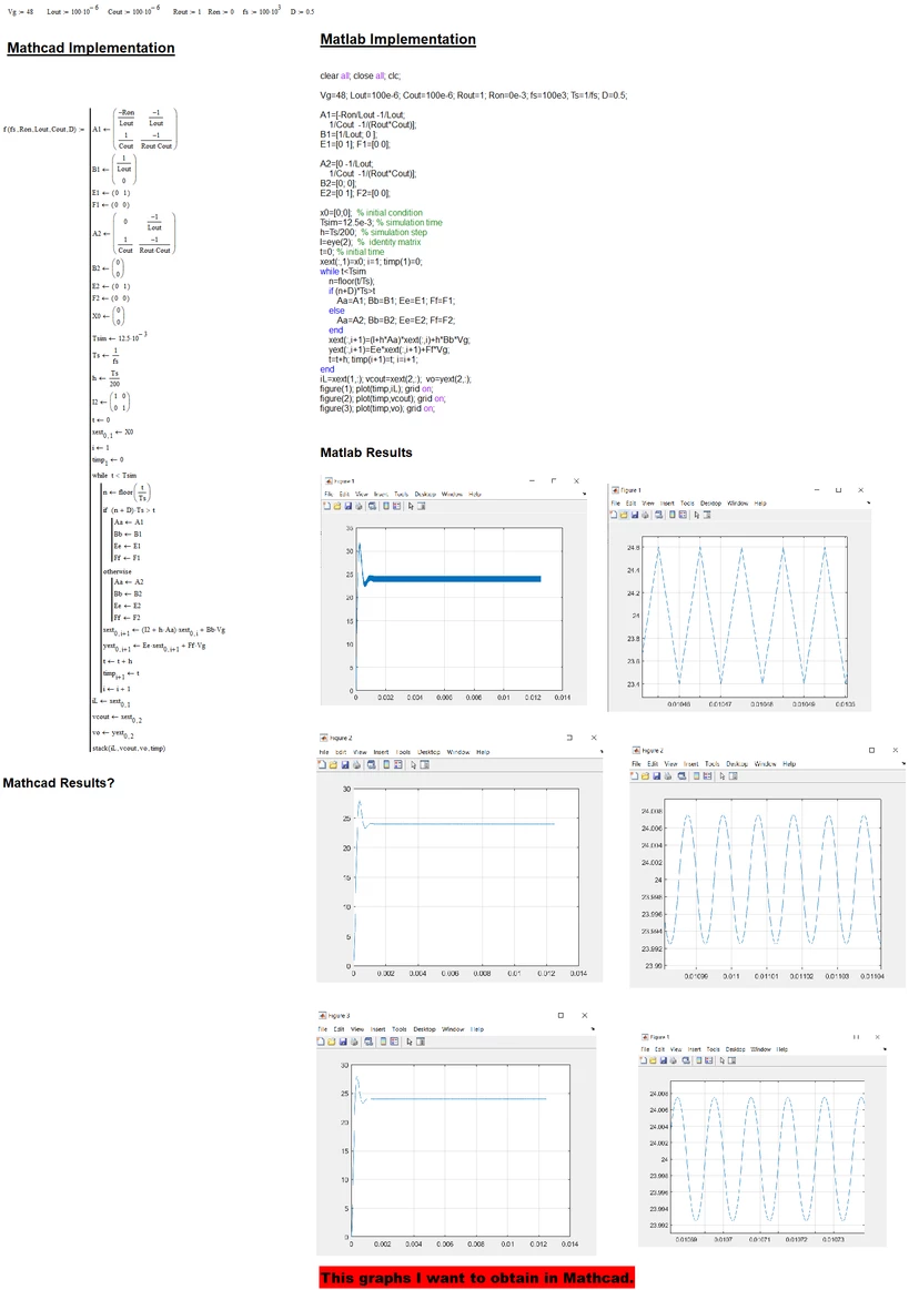
Can someone help me with this?

I want to translate some Matlab code into Mathcad 15.


CornelBejan_0-1618949224485.png


Thanks.

ACCEPTED SOLUTION

Accepted Solutions
Werner_E
25-Diamond I
(To:Werner_E)

I couldn't help trying it myself 😉

Here is a method without using F and yext and without using matrix/vector operation which does the full 250001 points calculation in less than one second. I made Tsim an argument of the function and added prec (aka precision) as its last argument. prec is responsible for the time step width h = Ts / prec. So prec=200 gives you the result from your Matlab screenshot. lower values result in a larger step width and less precision. With the new function you may also try prec=400 (resulting in 500001 points) without having to wait long for the result.
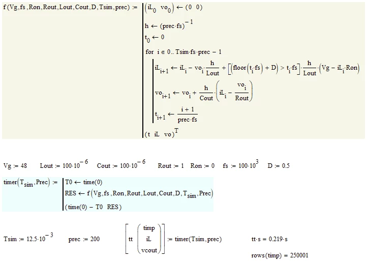
 

Werner_E_2-1619040121718.png


Guess I was wrong with respect to the plot points limit. This seems only apply when plotting a function over a range. When plotting one vector over the other, this limit seems not to apply as I also could plot vectors with more than 2 millions points.

I ran into a strange effect  (presumably round off errors when i tried to calculate the next time value using (i+1)*h. The values of iL were far off compared to the values calculated with the other methods (which resemble better the result of the MatLab calculation). Compare the two by changing the appropriate line in the program and decide yourself which result you may trust more - actually I am not really sure about it.

Here are the results which seem to match the Matlab results:
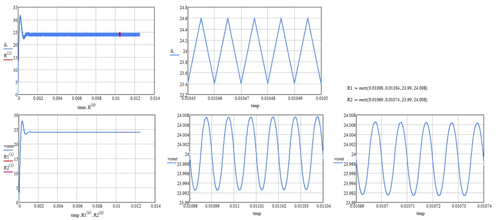
Werner_E_4-1619040246952.png


View solution in original post

14 REPLIES 14

Hi,

Nearly there just have to get the last variable "vo" sorted.  Must take a break to do something else.

Put in an iteration limit so easier to work with file.  Put in a trace on "i" to see the number of iterations in the debug window.

Here it is at 20000 iterations.  Confident "iL" and "vcout" are correct.

Capture.JPG

Cheers

Terry

Hi,

Finished file.  Have set the iteration number to 5.   The iteration number defines the number of plot points.  There is a limit in Prime to the number of points, much lower than Matlab.  In the example provided you will run out of plotting ability far before 12e-3 time limit.  It takes 25000 iterations for 1.25e-3.


View the debug window and set debugging and you can see how long it takes to get to the iteration limit set.


Capture.JPG


Cheers

Terry

Thanks.

For:

CornelBejan_2-1618997324356.png


CornelBejan_1-1618997309528.png


But it takes a long time to calculate and display the graphs ...
This is not very nice if you have to wait a few minutes for 1-2 graphs in the context of a simulation time quite short of a few milliseconds (for example 15-20 mili seconds)...
It would have been nice if it went faster and easier because if I put some graphs to calculate and display and for a relatively reasonable simulation time then my Mathcad will explode:)) ...

But anyway, thanks.

Werner_E
25-Diamond I
(To:Cornel)

I see no reason for the introduction of F1, F2, yext.
The output vectors vo and vcout seems to be the very same!?


Concerning Mathcads plot limitation:
Mathcad can show up to 500000 in one plot. Terrys function without his iteration limitation would make 250000 iterations (which takes about 20 Minutes on my old machine) and returns vectors with 250001 elements. So plotting iL or vcout over timp should be no problem. But when Terry tried to put iL and vcout together in one plot region, this makes up for 500002 points. Thats 2 points over the limit and so Mathcads throws an error.


But it takes a long time to calculate and display the graphs ...

Plotting itself should not take a long time as soon as the vectors are being calculated by the function f. But the latter really takes quite some time.

As I see it you have three ways out

1) Find a more efficient and faster way to do the calculations done in each iteration step. To begin with, you may start by deleting the calculation of "yext" as it looks like its unnecessary. You may also experiment with replacing the matrix/vector operations by simple operations with the appropriate scalars. This may blow up the code a little bit but should be faster.

2) Chose a smaller value for the simulation time Tsim. Basically this is exactly what Terrys iteration limitation does.

3) Chose a larger value  for the time step width h. Look at the calc time if you change the 200 there to just 20. But of course this is done at the cost of precision. You can see it if you compare the plots (especially the zoomed in views).


BTW, whats the calculation time in MatLab with the values your picture is showing?


Werner_E
25-Diamond I
(To:Werner_E)

I couldn't help trying it myself 😉

Here is a method without using F and yext and without using matrix/vector operation which does the full 250001 points calculation in less than one second. I made Tsim an argument of the function and added prec (aka precision) as its last argument. prec is responsible for the time step width h = Ts / prec. So prec=200 gives you the result from your Matlab screenshot. lower values result in a larger step width and less precision. With the new function you may also try prec=400 (resulting in 500001 points) without having to wait long for the result.


Werner_E_2-1619040121718.png


Guess I was wrong with respect to the plot points limit. This seems only apply when plotting a function over a range. When plotting one vector over the other, this limit seems not to apply as I also could plot vectors with more than 2 millions points.

I ran into a strange effect  (presumably round off errors when i tried to calculate the next time value using (i+1)*h. The values of iL were far off compared to the values calculated with the other methods (which resemble better the result of the MatLab calculation). Compare the two by changing the appropriate line in the program and decide yourself which result you may trust more - actually I am not really sure about it.

Here are the results which seem to match the Matlab results:

Werner_E_4-1619040246952.png


Cornel
19-Tanzanite
(To:Werner_E)

BTW, what's the calculation time in MatLab with the values your picture is showing?

About 4.174784 seconds.

Werner_E
25-Diamond I
(To:Cornel)


@Cornel wrote:

BTW, what's the calculation time in MatLab with the values your picture is showing?

About 4.174784 seconds.


Its nice to see that my variant is about twenty times faster 😉

Cornel
19-Tanzanite
(To:Werner_E)

@Werner_E: Yes.
But the idea is that the difference might be because in Matlab the algorithm is implemented with Forward Euler, and you implement by equations with differences.
Matlab may also decrease the time (I do not know exactly now if it would go down or not and I wouldn't want to pronounce yet) if it is implemented by your method, and not as it is initially implemented.
But it's ok in the way you implement it.

Can you explain a little bit how you thought about these lines?

CornelBejan_1-1619291950439.png

CornelBejan_2-1619291964157.png

The idea from the beginning was based on the Forward Euler algorithm.
I wanted to extend it to other algorithms, such as Runge Kutta or Gear.
But, as far as I can see, you chose to write equations with finite differences:

CornelBejan_4-1619292886774.png

I was thinking at one point about this variant with differences.
To see in the future, I will most likely come back with 1-2 examples at some point related to this method with differences because the method is interesting.


Werner_E
25-Diamond I
(To:Cornel)


@Cornel wrote:

Yes.
Can you explain a little how you thought about these lines?

CornelBejan_1-1619291950439.png


Tsim * fs * prec is the number of iterations your program is executing (in your program prec was 200). Its the number of times you can add h = 1/(fs*prec) to zero until you reach Tsim, which basically is what your program does. I needed this number because I turned your while-loop which was simply adding h until Tsim was reached, into a for loop. But I don't think that it will slow down the calculation if you stay with the while-loop, if you prefer.


But you, as far as I can see, chose to write equations with finite differences:


I simply took what you provided and made it much faster, thats all. I didn't change the algorithm you privided!

What we learned here is that matrix/vector operations are much slower than simple basic operations with scalars and when we have a program with a lot of iterations, that sums up in calculation time.

So whatever algorithm you try to implement, it may be a good idea to turn matrix operations done in the loops to basic operations with scalars.

Thats all there is to it.

Cornel
19-Tanzanite
(To:Werner_E)

CornelBejan_0-1619295043408.png

CornelBejan_1-1619295063213.png

I see the program running ok without even using:

CornelBejan_2-1619295126660.png

Is the purpose of these lines just to see how long it will take to run, calculate and display the implementation graphs, right?

Werner_E
25-Diamond I
(To:Cornel)


Is the purpose of these lines just to see how long it will take to run, calculate and display the implementation graphs, right?

Correct. Its a way to get the calculation time of a function. Its useful to see, which modification brings which speed advantage and how the precision argument prec and the simultion time Ts affect the calc time.

When I added that function I would not have thought that the modification would speed up the calc that significantly.

Cornel
19-Tanzanite
(To:Werner_E)

@Werner_E 


CornelBejan_1-1619353556750.png


1) The result of the graph below resulting from the above code represents the switched model. This is because the graph increases and decreases in a switching period (Ts = 1 / fs).


CornelBejan_3-1619353805986.png

The question would be what else should be added to the above code for the resulting graph to be the average of the switched graph?
Something like this:

CornelBejan_0-1619353525485.png

2) I would like to obtain as numerical values ​​the maximum value, the minimum value, and the average value, as shown in the second graph and not as shown in the first.

How could I do that?

CornelBejan_4-1619354098451.png

CornelBejan_5-1619354287289.png

3)  The first graph starts from 0 to Tsim.
How could I get the graph to start not from 0, but from another value greater than 0 (as shown in the second graph).

CornelBejan_6-1619354445860.png

CornelBejan_7-1619354474747.png


CornelBejan_9-1619354626198.png


Werner_E
25-Diamond I
(To:Cornel)

ad 1) Not sure what exactly you are looking for. I had not looked at your algorithm or model, I simply speeded it up.

ad 2) I see no way to achieve what you would like to see. Awkward workaround could be to overlay an evaluation region. type max(iL)= and drag that region near or over the plot. Sure not convenient

ad 3) Simply change the values on the x-axis in the plot.

Cornel
19-Tanzanite
(To:Cornel)

@LucMeekes@Werner_E 

Do you have any idea???

Announcements

Top Tags