Community Tip - You can subscribe to a forum, label or individual post and receive email notifications when someone posts a new topic or reply. Learn more! X
- Subscribe to RSS Feed
- Mark Topic as New
- Mark Topic as Read
- Float this Topic for Current User
- Bookmark
- Subscribe
- Mute
- Printer Friendly Page
No name curve
- Mark as New
- Bookmark
- Subscribe
- Mute
- Subscribe to RSS Feed
- Permalink
- Notify Moderator
No name curve
We have:
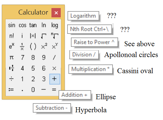
a+b - Video Link : 2089
a-b - Hyperbola
a*b - Cassini oval
a/b - Apollonian circles
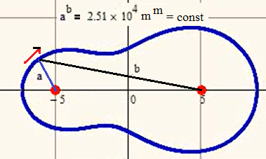
a^b - see above. Do you know the name of this fine curve?
- Mark as New
- Bookmark
- Subscribe
- Mute
- Subscribe to RSS Feed
- Permalink
- Notify Moderator
- Mark as New
- Bookmark
- Subscribe
- Mute
- Subscribe to RSS Feed
- Permalink
- Notify Moderator
- Mark as New
- Bookmark
- Subscribe
- Mute
- Subscribe to RSS Feed
- Permalink
- Notify Moderator
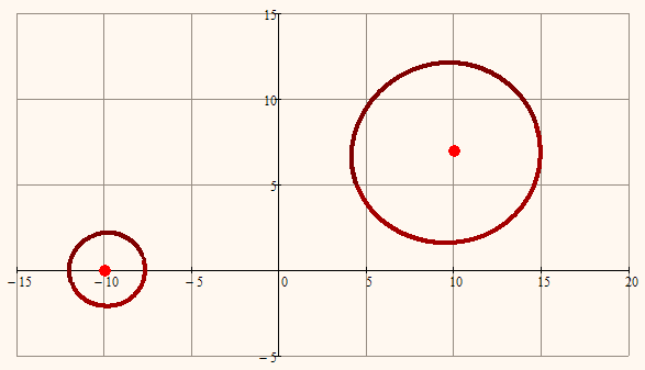
Are you sure about your equations?
Here is what I get using the same "focal" points and the same a^b value (10^7):
- Mark as New
- Bookmark
- Subscribe
- Mute
- Subscribe to RSS Feed
- Permalink
- Notify Moderator
- Mark as New
- Bookmark
- Subscribe
- Mute
- Subscribe to RSS Feed
- Permalink
- Notify Moderator
For better reliability and quality here the same animation as attachment
- Mark as New
- Bookmark
- Subscribe
- Mute
- Subscribe to RSS Feed
- Permalink
- Notify Moderator
Thanks, Werner.
But we must convert avi into mov, for example.
And second an main - a^b must be const. Show please a and b. Is it ovals Cassini?
- Mark as New
- Bookmark
- Subscribe
- Mute
- Subscribe to RSS Feed
- Permalink
- Notify Moderator
> But we must convert avi into mov,
So thats the reason the embedded video of mine doesn not work and is showing the "This video is not available"?
Shame on PTC for providing such a lousy platform!
But anyway I prefer a file which I can download, play locally using a player of my choice, being able to step back and forth frame by frame, take snapshots, etc.
The flash streaming player provided here does not offer that functionality and ever so often chokes and fails.
> And second an main - a^b must be const.
Thats exactly whats the case. a is the distance of a point of the curce from the left red "focal" point and b is the distance from the right one
> Show please a and b
My animation is not animation one specic curve point for point but the animation is showing the different shapes when the constant a^b changes. So I could add the distances and the value of a^b for just a few arbitrary selected points whoích would prove and show nothing.
> Is it ovals Cassini?
No, but they remind somehow on Cassini. Don't know if this familiy of curves was given a specific name.
Its the very same curve you started this thread, but the curve your animation is showing looks a bit strange to me and differs from mine. I posted a picture of the curve using your values an got a different shape. Wonder if the error is in my sheet or in yours. But then - its not that important, but its nice to play with.
WE
- Mark as New
- Bookmark
- Subscribe
- Mute
- Subscribe to RSS Feed
- Permalink
- Notify Moderator
Thanks!
But it will be good to show one more animation

- Mark as New
- Bookmark
- Subscribe
- Mute
- Subscribe to RSS Feed
- Permalink
- Notify Moderator
ValeryOchkov написал(а):
Thanks!
But it will be good to show one more animation
- Mark as New
- Bookmark
- Subscribe
- Mute
- Subscribe to RSS Feed
- Permalink
- Notify Moderator
Hi. I'm not a particular entusiast of animations. Or not good doing that, perhaps. This example is more simple because take the origin as one focus. The expression for the discriminant is very complicated, can't see any pattern.
Best regards.
Alvaro.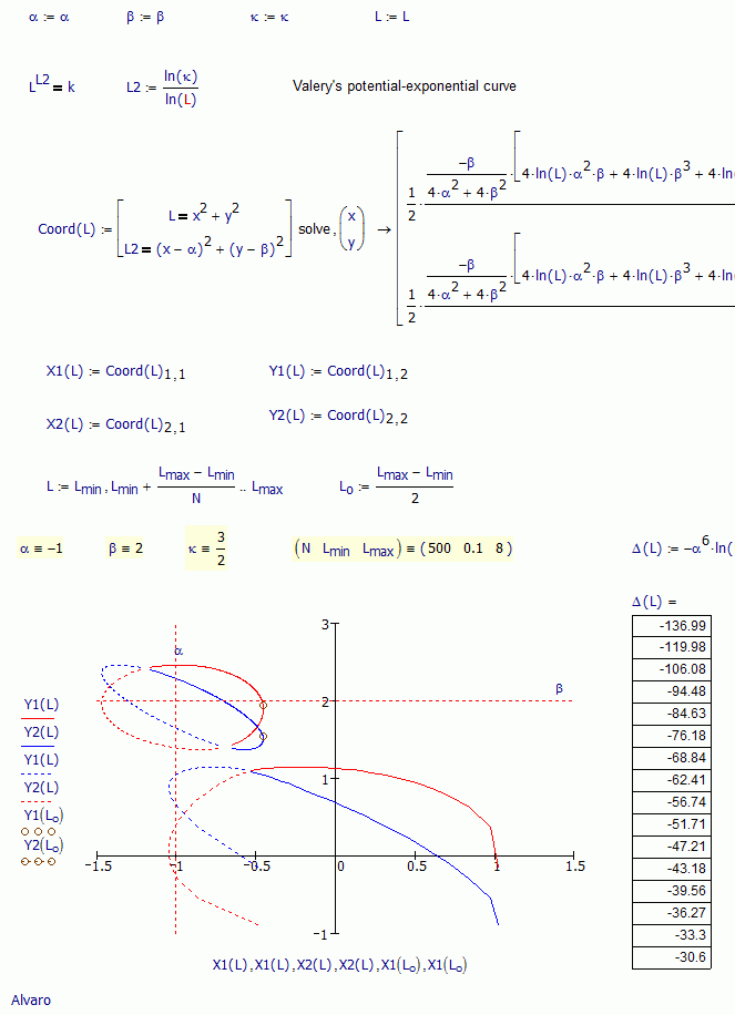
- Mark as New
- Bookmark
- Subscribe
- Mute
- Subscribe to RSS Feed
- Permalink
- Notify Moderator
- Mark as New
- Bookmark
- Subscribe
- Mute
- Subscribe to RSS Feed
- Permalink
- Notify Moderator

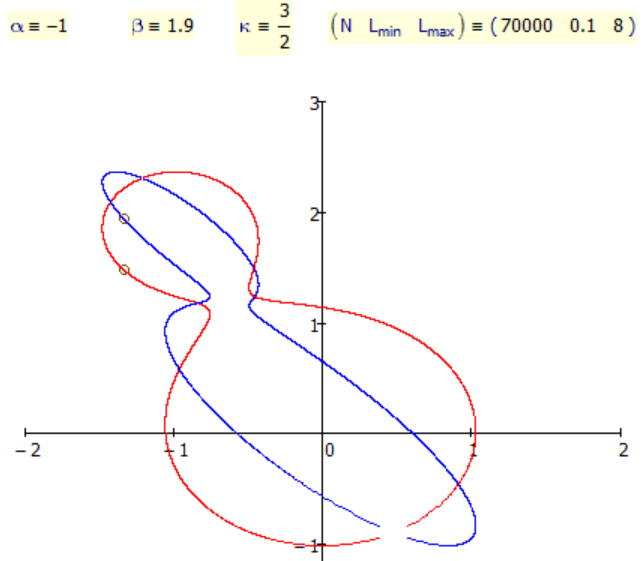
Shouldn't it be L^2 and L2^2 ?
Furthermore I don't understand why you combine X1 with Y2 and X2 with Y1 in your plot!?
The intersection of the two circles are just (X1/Y1) and (X2/Y2)
Regards
Werner
- Mark as New
- Bookmark
- Subscribe
- Mute
- Subscribe to RSS Feed
- Permalink
- Notify Moderator
Werner Exinger wrote:
Shouldn't it be L^2 and L2^2 ?
Yes, you're right. That's was an attemp to see if there are somplification about Discriminant, but aren't, only appear L instead L^2. The measured distances, in that case, are sqrt(L) and sqrt(L2), and must to correct also the constant k. But the general arrange is the same.
Werner Exinger wrote:
Furthermore I don't understand why you combine X1 with Y2 and X2 with Y1 in your plot!?
To see which or if there are strange solutions, introduces by the algebraic manupulations isolating x and y. Without polar representation of the curves, and with that complicated discriminant, I don't see which points could be "strange solutions". Notice that in the interval there are a lot of negative Delta values that carry complex values for x and y.
Best regards.
- Mark as New
- Bookmark
- Subscribe
- Mute
- Subscribe to RSS Feed
- Permalink
- Notify Moderator
> I don't see which points could be "strange solutions". Notice that in the interval there are a lot of negative Delta values that carry complex values for x and y.
I still don't see the reason for combining the absicissa from one solution with the ordinate of the second. Points derived that way aren't solutions. And yes, a lot of values for L would produce non-real values for L2 - Thats slowing down calculation and plotting a bit but I found no (quick) way to determine the valid range for the first distance L depending on the constant C (kappa in your sheet) and the distance between the two "focals".
Here is what I get using your sheet without combining coordinates from different points of intersections and its definitely not a quartic but of higher order than four, if its algebraic at all. I scaled to get equal scale on both axis as at first I was confused why the plot is not symmetrical according to the line through the two "focals" 😉

Regards
Werner
- Mark as New
- Bookmark
- Subscribe
- Mute
- Subscribe to RSS Feed
- Permalink
- Notify Moderator
Hi Werner. Thanks for the attached.
"Strange solutions" are those introduced by some algebraic manipulations in the process of isolating variables. For example, from
x-1 = sqrt(3-3x),
you can get
x^2-2x+1 = 3-3x,
then
x^2+x-2=0
which gives x=-2 and x=1. But actually, x=-2 is a "strange solution" introduced by the algebraic manipulation, because don't hold the original equation, and must to be discarded. The only one solution for the original equations is x=1. Maple or mupad solution seems to not introduce those strange solutions. But this must to be, maybe if not full prove, but analyzed at least.
About the complexes values, the "quick" way to prevent them, or, better say, the domain for x, is with the discriminant, i.e. the under radical expression, the Delta(L) in the worksheet. But complex, and function of all other variables: alpha, beta, L, kappa. With a for loop can evaluate it, stored in an intermediate variable for speed the calculations, and continue with x, y1, y2 only when Delta(L) > 0. But that's for speed. Let's the machine do that inutile work.
About x1 vs y1,y2 or x2 vs y1,y2, remember that in geometry, unlike calculus, x and y are equivalents. I don't want to discard x2 prematurely.
Best regards.
Alvaro.
- Mark as New
- Bookmark
- Subscribe
- Mute
- Subscribe to RSS Feed
- Permalink
- Notify Moderator
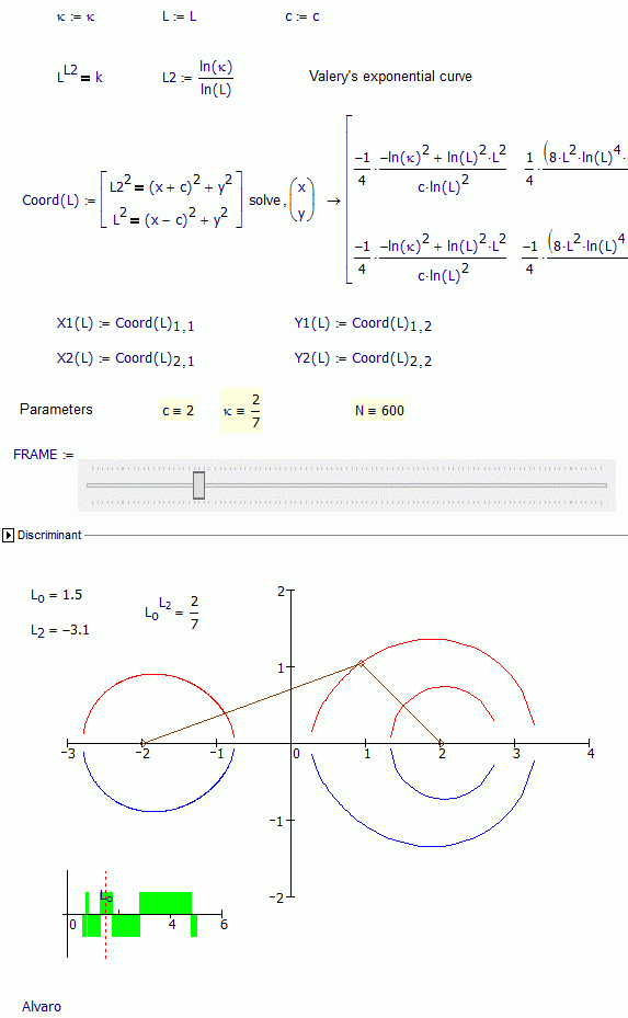
More easy setup, assuming line between focus as y=0, and symetric about the origin. Can be rotated and translated later for general case. For this, Delta have more sense, and can find roots. Unfortunatelly, mupad don't give all roots for the discriminant, only one. So, MC11 better.
Parametrizacion as function of L, canonical parametrization along s = arc length too complicated, can't simplify the integral yet.
Path with holes, aren't analityc. Bye bye complex variable tools. So, imaginary nor algebraic representation could take some time.
For better plots, adaptive steps must neede, like the routines in Amazing Images ebook.
Best regards.
Alvaro.
- Mark as New
- Bookmark
- Subscribe
- Mute
- Subscribe to RSS Feed
- Permalink
- Notify Moderator
- Mark as New
- Bookmark
- Subscribe
- Mute
- Subscribe to RSS Feed
- Permalink
- Notify Moderator
Attached a mc15 worksheet, saved as mc11, with some "easy" (most precisely, simmetrical) expressions for the discriminant, polar and others properties of the Valery's exponential curve.
Best regards.
Alvaro.

