Pulse function

---

@LucMeekes wrote:

Worksheet(s) please...!

 

Luc

---

Here you are

I did no exact timing but it looks to me like calculations need much more time in Prime than in MC15

BTW, omitting the vertical line segments in a step function would be perfectly correct from a mathematical point of view but I understand that its undesirable for an engineer.

There is a simple cure, though.

My suggestion of a step width of 0,01 ms in the range was far too low. It should read 0.01 s which is good enough for the plots.

The range 0s, 0.01ms .. 4.2s forces the plot to be evaluated at 4.2 * 10^5 positions. Mathcad could handle that many points (nearly half a million) but Prime seems to have different limits and it falls back to this strange looking plot where you could not change anything (line style, thickness, .. ) other than the colour.

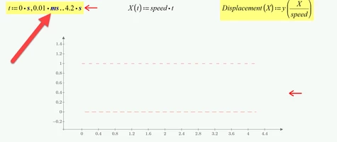
Changing the range to read 0s,0.01 s .. 4.2 s gives us 421 points which is more than enough for this simple rectangular function. Changing the step width to 1 ms for 4201 points should be OK, too, of course.

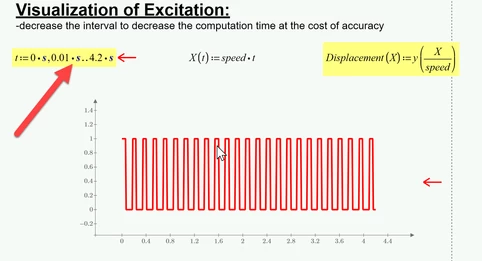
Even simple 2D plots always were one of the many drawbacks in Prime and PTC was not able or willing to improve it. You may have noticed that there are not axis labels, no grid lines, the possibilities to customize the plot are much more limited and simple things like changing the axis limits are much more cumbersome.

In Prime 5 PTC has introduced a third party diagram component (look at the "calculate" ribbon for it). I don't like this add-on as its very slow and laborious to handle, does not scale correctly when used with a high resolution 4K display (making it nearly unusable) and does not support units (a no-go in a program like Mathcad/Prime).

Nonetheless, if you decide that you like Prime despite its drawbacks, you may give this plot component a try, too.