Community Tip - Stay updated on what is happening on the PTC Community by subscribing to PTC Community Announcements. X
- Subscribe to RSS Feed
- Mark Topic as New
- Mark Topic as Read
- Float this Topic for Current User
- Bookmark
- Subscribe
- Mute
- Printer Friendly Page
FFT peak amplitude
- Mark as New
- Bookmark
- Subscribe
- Mute
- Subscribe to RSS Feed
- Permalink
- Notify Moderator
FFT peak amplitude
Hello,
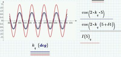
In the attached worksheet, the FFT of a function is calculated. I would like to get the amplitude at each of the frequencies from the signal. From the plots of the FFT magnitude at various frequencies, it can be seen that the peaks amplitude decrease with increasing the frequency. The plots also show that sometimes the first peak is larger than the second peak and sometimes it is reversed.
I was wondering if this is a natural behavior of FFT or I must modify the script. I greatly appreciate your advice.
All the best,
Payman
Solved! Go to Solution.
Accepted Solutions
- Mark as New
- Bookmark
- Subscribe
- Mute
- Subscribe to RSS Feed
- Permalink
- Notify Moderator
There are a number of different things going on here, and too many complications in the worksheet to let the basic issues show clearly. I didn't change most of the sheet, but I did remove the second delta 1 frequency term, since it just clouds the issue.
1. The cases of z= 5 and z=500 show the same symptom: leakage. Due to the spacing of the sampling intervals, integer z does not correspond to integer # of cycles over the full sampling period.I added some functions in rev2 (attached) to calc power and actual bin number. z=5 is centered at bin 4.69, z=500 is centered at bin 469.19. the different fractional spacing explains the difference in spectral component amplitudes - leakage is spread differently.
2. When z=0.1 (low) , the actual value of the sampled function is near 0, not 1, since the sampling does not start at zero argument of the cosine, since k has an initial offset. Not sure why this is need, since the spectrum depends only on the span of the sampled data, not the origin. In any case, the waveform for z = 0.1 is around the zero crossing of the cosine, not near its peak.
3. When z =0, the sampled function is constant=1, giving only a bin(0) value = 1, the average (only thing present). When z is not zero, the cosine consists of two complex exponential components, each of amplitude 1/2, one at bin# = z and one at bin# = -z, which shows up at bin# = N-z since the spectrum is effectively periodic with N, the # of samples.moving from z=0 to z not 0 results in switching from one component with value 1 to two components of value 1/2 each. The FFT returns only one of these. You have to reconstruct the other.
The FFT assumes a real input, and returns only that part of the spectrum from 0 to fs/2. It does not return the upper half (fs/2 to fs) of the full spectrum, since these values are complex conjugates of the lower half. However, these missing values need to be included in any power calc.The CFFT function works with complex as well as real input waveforms, and returns the complete spectrum, with all components from 0 to fs. It works with any size vector. Unless dealing with a large # of transforms, I personally find the simplicity of using the CFFT worthwhile.
I think your worksheet is much too complicated to serve as a vehicle to explore DFT behavior. The best way to familiarize yourself with how the DFT functions behave is to work with a simple function - one real sinusoid, or even better, a single complex exponential. since the all the DFT's are linear. Learning how a single component works should help with more complicated behavior. Deal with sample #'s first and then set up with time and frequency. Keep track of how many cycles are in the complete sampling interval - this is the effective bin#. Note that if the input is sampled at k=0,1,2,...9, that the repeat sample span is 10, since this is assumed to be the same as k=0. the repeat interval is not 9.
Hope this helps,
Lou
- Mark as New
- Bookmark
- Subscribe
- Mute
- Subscribe to RSS Feed
- Permalink
- Notify Moderator
You need to read the Mathcad 15 help files on CFFT and FFT.
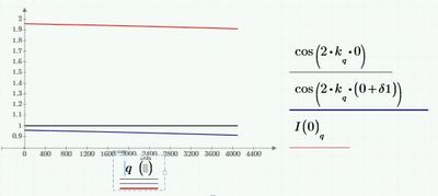
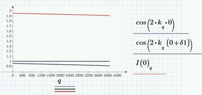
FFT and fft require a sample size that's a power of 2 long. CFFT and cfft do not; any length is okay. You did it right, 4096 samples. But the amplitudes you're reporting are not correct. Your first plot is I(0), if I break down the individual parts, then ploy the sum, we get:
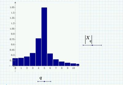
and you report the fft as
The first spike (the steady-state component) should be nearly 2, but reports as ~1, because of the way FFT scales its results (fft is different!) So fix that first.
I suspect that the reason the amplitude magnitudes switch around has to do with the phase relationship of the signals and the fact that you have a very short sample size.
- Mark as New
- Bookmark
- Subscribe
- Mute
- Subscribe to RSS Feed
- Permalink
- Notify Moderator
Hi,
FFT must be supplied with a vector consisting of, for example, samples of a continuous function. The function must be sampled respecting the sampling theorem, that is, you need to know the sampling frequency. In your case the FFT argument is a function which in turn has only an independent variable z0 as its argument. In the function, however, the k that varies with q is also present. It does not seem to me that FFT receives an array of samples, but does what it can and returns what it can. An example of how you should proceed is the following:
Then, to know the amplitudes of the harmonics you can use the sliders as in the following figure relating to an IQ-QPSK signal:
- Mark as New
- Bookmark
- Subscribe
- Mute
- Subscribe to RSS Feed
- Permalink
- Notify Moderator
Can you save your file as an mcd11 version file and post that?
Thanks,
Lou
- Mark as New
- Bookmark
- Subscribe
- Mute
- Subscribe to RSS Feed
- Permalink
- Notify Moderator
- Mark as New
- Bookmark
- Subscribe
- Mute
- Subscribe to RSS Feed
- Permalink
- Notify Moderator
What is happening is called spectral "leakage." This occurs when the total sampling period (based on N sampling segments, not N-1) does not contain an integer number of cycles of the input sinusoidal component. For example, if the input x(k) has 5 periods (freq = 5) over the full sampling interval, then the DFT sample X(5) will have the expected value, and the remaining components will be zero. If the input freq is 5.5, then the DFT in the two adjacent integer bins, X(5) and X(6) will be equal, and approximately 0.64 of the expected value. A number of other adjacent coefficients will also be nonzero.
In the attached rev of your file, I added a plot that shows both spectral components offset and expanded, so the nearby components are more visible. Both show leakage, and the power is spread over multiple DFT components, so that none of these gives the true amplitude of of the input sinusoid. When the actual input frequency falls directly on a DFT bin, then one gets a single true component. You can try some of the other suggested values to see the effects of leakage and when it is not present.
The other file shows the leakage components come from sampling a sinc-like function at integer values. for the case where the input freq is an integer, the zero, the only nonzero value is at the input frequency. If the input freq is not an integer, then all samples are nonzero, falling off only as 1/n away from the center frequency.
I like to visualize this from the viewpoint that the DFT is a Fourier series of a sampled, periodic-in-time, input signal. SInce the input is sampled, its spectrum - the DFT - repeats, the DFT being just one period. Piecing the input together for more than one period shows why the spectrum is not that of a single sinusoid. The attached pdf shows three periods of a sinusoid that has 2.1 cycle in each sampling period.
One way to reduce leakage and have non-integer frequencies show up with less magnitude distortion is to use windowing. This effectively provides a different function that gets sampled for the DFT coefficients, replacing the sinc-like function with something flatter over a bin width. The tradeoff is that the frequency resolution is usually worse.
Lou
- Mark as New
- Bookmark
- Subscribe
- Mute
- Subscribe to RSS Feed
- Permalink
- Notify Moderator
Hi LouP,
Thank you very much for your descriptive reply. From your examples, I realized the effect of the frequency leakage on the spike's amplitude and I'll add window function to mitigate the impact.
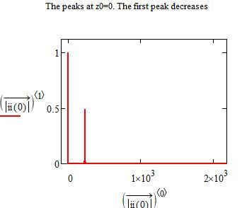
There is a point still not clear to me. When z0=0, the first spike amplitude is near 1 but for any nonzero value of z0 this amplitude's value drops significantly (almost by half). Could you please give me a hint to understand the reason. From my understanding, the frequency leakage could not make such a strong impact, I guess.
I appreciate your time and consideration.
Payman
- Mark as New
- Bookmark
- Subscribe
- Mute
- Subscribe to RSS Feed
- Permalink
- Notify Moderator
When z0 = 0, the equation defaults to I(0) := 1 + cos(2 k d1), which, over the small area you're sampling is a very slowly varying function. Plotting the two components and the function:
When you take the FFT, we get:
So you can see that for the slowly varying (nearly constant function, the zeroth coefficient of the FFT (which is the steady state or average value) is most of the value. As z0 grows the functions vary more rapidly and the leakage is more pronounced: I(5) below!
- Mark as New
- Bookmark
- Subscribe
- Mute
- Subscribe to RSS Feed
- Permalink
- Notify Moderator
Hi Fred,
Thank you very much. I would like to compare the two cases here when z0=5 and z0=500. Although the frequency difference is large, the amplitudes differ slightly. For example, the first spike's amplitude at z0=5 is 0.41 and at z0=500 is 0.47.
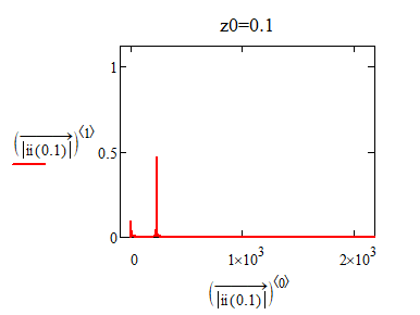
There is another interesting case when z0=0.1 (see the below plot !!!)
Even applying window cannot help with this example. I think the reason should be somewhere else than increasing the frequency.
I appreciate your help and consideration,
Payman
- Mark as New
- Bookmark
- Subscribe
- Mute
- Subscribe to RSS Feed
- Permalink
- Notify Moderator
Okay, It took a bit (I've only got Prime Express).
Attached are two files:
- fft review.mcdx, a Prime 4.0 file (openable with any later Prime)
- fft review.pdf a readable (I hope) version of that file
Comments are in the files--I hope this answers your questions.
- Mark as New
- Bookmark
- Subscribe
- Mute
- Subscribe to RSS Feed
- Permalink
- Notify Moderator
There are a number of different things going on here, and too many complications in the worksheet to let the basic issues show clearly. I didn't change most of the sheet, but I did remove the second delta 1 frequency term, since it just clouds the issue.
1. The cases of z= 5 and z=500 show the same symptom: leakage. Due to the spacing of the sampling intervals, integer z does not correspond to integer # of cycles over the full sampling period.I added some functions in rev2 (attached) to calc power and actual bin number. z=5 is centered at bin 4.69, z=500 is centered at bin 469.19. the different fractional spacing explains the difference in spectral component amplitudes - leakage is spread differently.
2. When z=0.1 (low) , the actual value of the sampled function is near 0, not 1, since the sampling does not start at zero argument of the cosine, since k has an initial offset. Not sure why this is need, since the spectrum depends only on the span of the sampled data, not the origin. In any case, the waveform for z = 0.1 is around the zero crossing of the cosine, not near its peak.
3. When z =0, the sampled function is constant=1, giving only a bin(0) value = 1, the average (only thing present). When z is not zero, the cosine consists of two complex exponential components, each of amplitude 1/2, one at bin# = z and one at bin# = -z, which shows up at bin# = N-z since the spectrum is effectively periodic with N, the # of samples.moving from z=0 to z not 0 results in switching from one component with value 1 to two components of value 1/2 each. The FFT returns only one of these. You have to reconstruct the other.
The FFT assumes a real input, and returns only that part of the spectrum from 0 to fs/2. It does not return the upper half (fs/2 to fs) of the full spectrum, since these values are complex conjugates of the lower half. However, these missing values need to be included in any power calc.The CFFT function works with complex as well as real input waveforms, and returns the complete spectrum, with all components from 0 to fs. It works with any size vector. Unless dealing with a large # of transforms, I personally find the simplicity of using the CFFT worthwhile.
I think your worksheet is much too complicated to serve as a vehicle to explore DFT behavior. The best way to familiarize yourself with how the DFT functions behave is to work with a simple function - one real sinusoid, or even better, a single complex exponential. since the all the DFT's are linear. Learning how a single component works should help with more complicated behavior. Deal with sample #'s first and then set up with time and frequency. Keep track of how many cycles are in the complete sampling interval - this is the effective bin#. Note that if the input is sampled at k=0,1,2,...9, that the repeat sample span is 10, since this is assumed to be the same as k=0. the repeat interval is not 9.
Hope this helps,
Lou
- Mark as New
- Bookmark
- Subscribe
- Mute
- Subscribe to RSS Feed
- Permalink
- Notify Moderator
- Mark as New
- Bookmark
- Subscribe
- Mute
- Subscribe to RSS Feed
- Permalink
- Notify Moderator
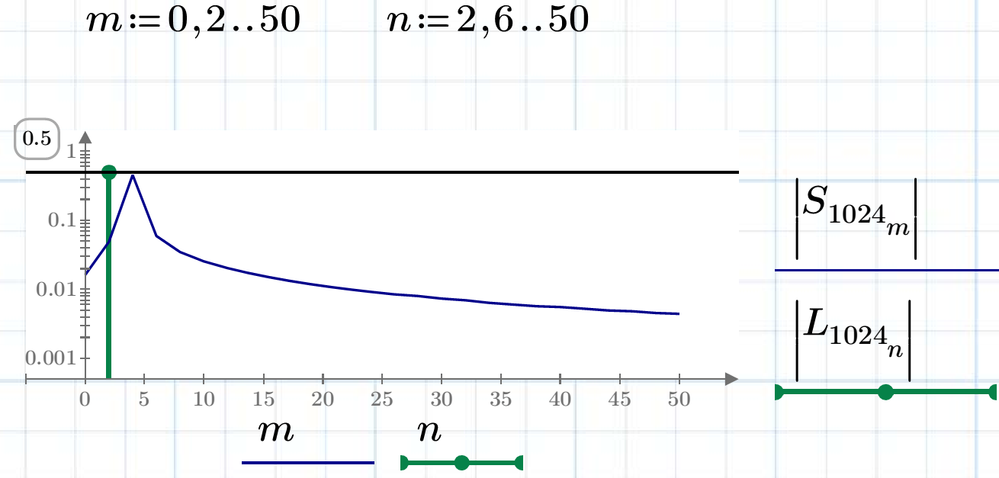
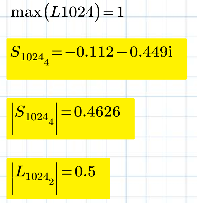
linterp can make true values of signal spectrum magnitude without edge spectrum.
- Tags:
- Electric_circuit
- Mark as New
- Bookmark
- Subscribe
- Mute
- Subscribe to RSS Feed
- Permalink
- Notify Moderator
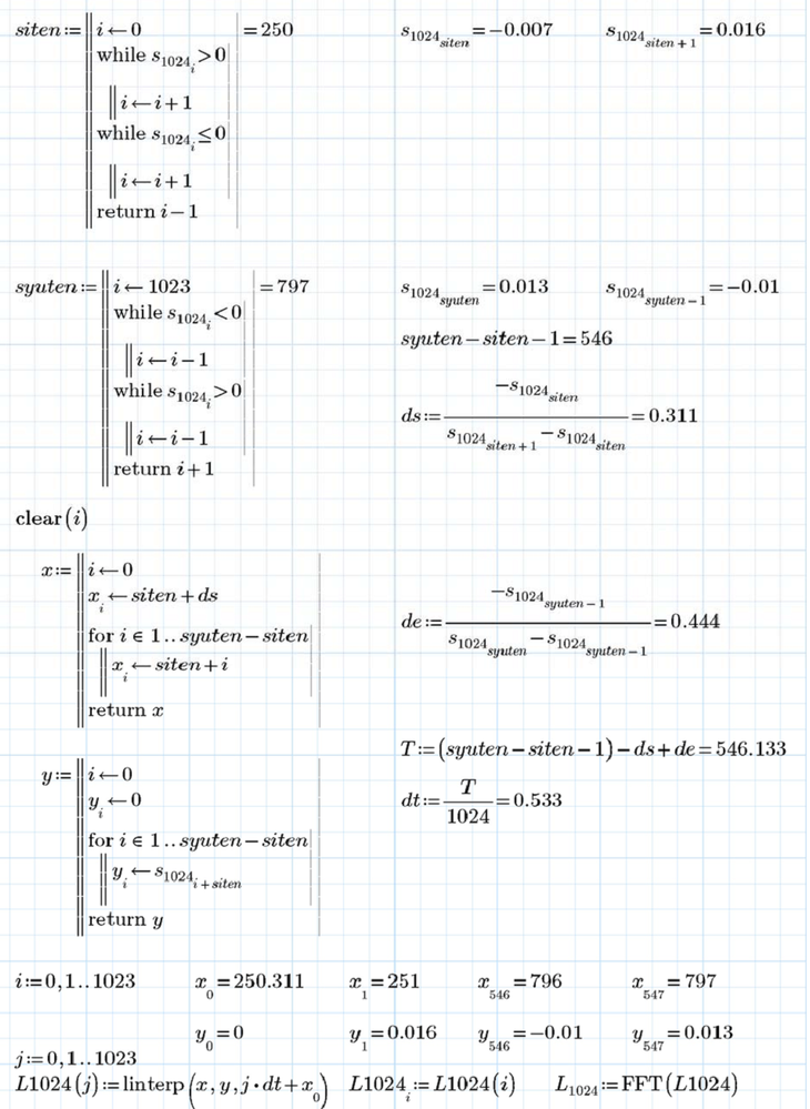
Thank you very much. Could you please define "L1024"?
Payman
- Mark as New
- Bookmark
- Subscribe
- Mute
- Subscribe to RSS Feed
- Permalink
- Notify Moderator
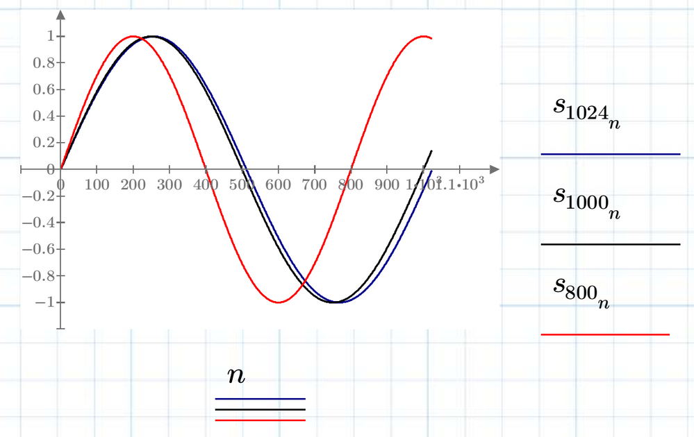
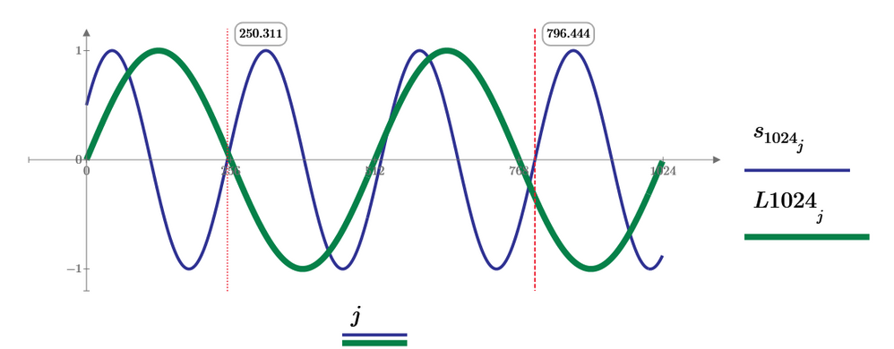
x,y is original signal data of 2 cycles from 250 to 797 as shown by blue line.
j*dt+x0 is the jth linear interpolation data time of 1024 linterp data as shown by green line.
dt is the new sampling rate of green line data. In this case, new interpolated data have two cycles.
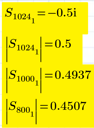
Therefore, the fundamental spectrum of this signal is L1024[2. It is 0.5, the half of signal magnitude.
- Tags:
- Electric_circuit


