Community Tip - Want the oppurtunity to discuss enhancements to PTC products? Join a working group! X
- Subscribe to RSS Feed
- Mark Topic as New
- Mark Topic as Read
- Float this Topic for Current User
- Bookmark
- Subscribe
- Mute
- Printer Friendly Page
Two Square Wave Vibration Examples
- Mark as New
- Bookmark
- Subscribe
- Mute
- Subscribe to RSS Feed
- Permalink
- Notify Moderator
Two Square Wave Vibration Examples
Hi,
Given the recent posts on the forum, I was curious to try and drive a mass, spring, damper system using a square wave. Luc posted an interesting solution for creating a square wave. There are decent quick sheets for mass, spring, damper systems in Mathcad 15. So I just combined the two things. I did have to modify the square wave definition some. The state space solver is faster and more robust. However, using odesolve provides a check. Working with each solver is different. The examples help show how to work with each solver.
The examples allow you to see what happens when you use a square wave instead of a cosine wave. Also, what happens when the square wave duty cycle changes. You can see that traditional ode solutions don't match reality. I've seen this before as well. The classic text book solutions are limited in a number of ways.
Also, thanks to the other forum members who helped me create these examples. I couldn't have did it without their help.
Anthony
Update; Added additional information and fixed some bugs. Also added pdf files of the examples.
- Labels:
-
Mathcad Usage
- Mark as New
- Bookmark
- Subscribe
- Mute
- Subscribe to RSS Feed
- Permalink
- Notify Moderator
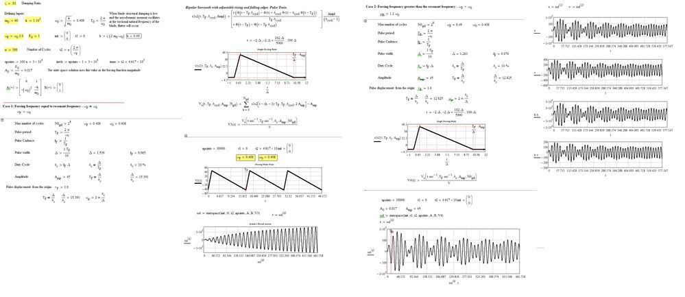
I have adapted your data to a sawtooth excitation with an adjustable duty cycle. What do you think?
- Mark as New
- Bookmark
- Subscribe
- Mute
- Subscribe to RSS Feed
- Permalink
- Notify Moderator
that's really cool. i love the response you got there.
- Mark as New
- Bookmark
- Subscribe
- Mute
- Subscribe to RSS Feed
- Permalink
- Notify Moderator
i looked into the slow down, when working with the odesolve output. i was able to prove it had to do with taking derivatives of the function output. the forum won't let me edit my original post. so i have attached the new files to this post. i have optimized versions, which run fast and manually calculate velocity, kinetic energy, acceleration, and the reaction forces. the trick is to use matrix output and do the calculations yourself. rather than taking derivatives of the function output. you see the slow down when setting the number of cycles to 300, using the comparison files. i had to switch the number of cycles to 10, so that the pdf files were manageable. the reason for 300 cycles is that it allows you to compare to the classical magnification/amplitude factor.
- Mark as New
- Bookmark
- Subscribe
- Mute
- Subscribe to RSS Feed
- Permalink
- Notify Moderator
You can edit, up to about a day, maybe two, after initial post.
After that, the best option is to attach a reaction/reply; which is what you did..
Success!
Luc
- Mark as New
- Bookmark
- Subscribe
- Mute
- Subscribe to RSS Feed
- Permalink
- Notify Moderator
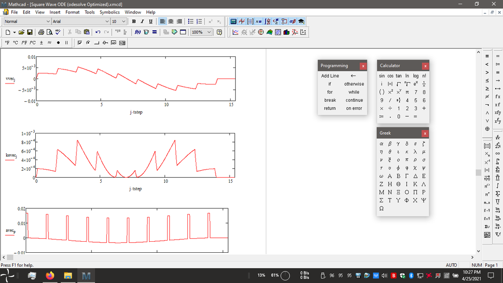
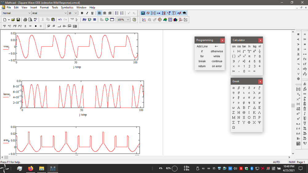
i am working on some changes to make it easier to work with beats. this was an input type posted by a different user earlier. i was looking at resonance and he was looking at beats. the file isn't finished yet, but i got a wild response while testing random inputs. check this out. pretty crazy. those are velocity, kinetic energy, and acceleration. the kinetic energy plot is the wildest looking one. i'll post updated files once i get them done.
- Mark as New
- Bookmark
- Subscribe
- Mute
- Subscribe to RSS Feed
- Permalink
- Notify Moderator
lol, here is another. i wouldn't want to ride on an elevator with this acceleration curve. it would probably make for a good amusement park ride though.
- Mark as New
- Bookmark
- Subscribe
- Mute
- Subscribe to RSS Feed
- Permalink
- Notify Moderator
here are updated files. they make it easier if you want to look at beats. i put them in a zip file. there are no pdfs this time around. the files are for MC15 only.
- Mark as New
- Bookmark
- Subscribe
- Mute
- Subscribe to RSS Feed
- Permalink
- Notify Moderator
i was playing around with inputs and found a bug in state space. in the help it says one of the inputs to the solver is intvls. however, it is actually npoints. using intvls incorrectly changes the time step. intvls is an optional input to odesolve. however, i found it wasn't doing anything, so i took it out of there. odesolve doesn't have the problem of changing time step.
one other thing i found is you get more ability to look at overdamped systems with odesolve. state space starts having problems when the damping ratio is greater than about 10. you can go up to 10,000 with odesolve. i didn't check beyond 10,000. but odesolve seems to work better for overdamped systems.
i made some slight changes to things, looking into this. i also added average calculations for some inputs. the average i calculate is for the appropriate matrix locations. the mean function in mathcad calculates the whole matrix. so it takes several zero locations into the calculations, which isn't right. the zero locations were never calculated in the first place. so plenty of quirks going on.
- Mark as New
- Bookmark
- Subscribe
- Mute
- Subscribe to RSS Feed
- Permalink
- Notify Moderator
hi,
attached are updates of the two examples. i found that the help for the state space and odesolve solvers has some problems. through experimentation, i found inputs to the solvers that output the correct time step and run out to the max time. the attachments fix these problems. the key thing to do, when using either of these solvers, is to check that the displacement calculations are output at the correct time step and run out to the max time. i changed all of my manual calculations, that use the solver displacement output, to work with the updated output. hopefully, everything is right now. if you find a problem, let me know.
anthony
- Mark as New
- Bookmark
- Subscribe
- Mute
- Subscribe to RSS Feed
- Permalink
- Notify Moderator
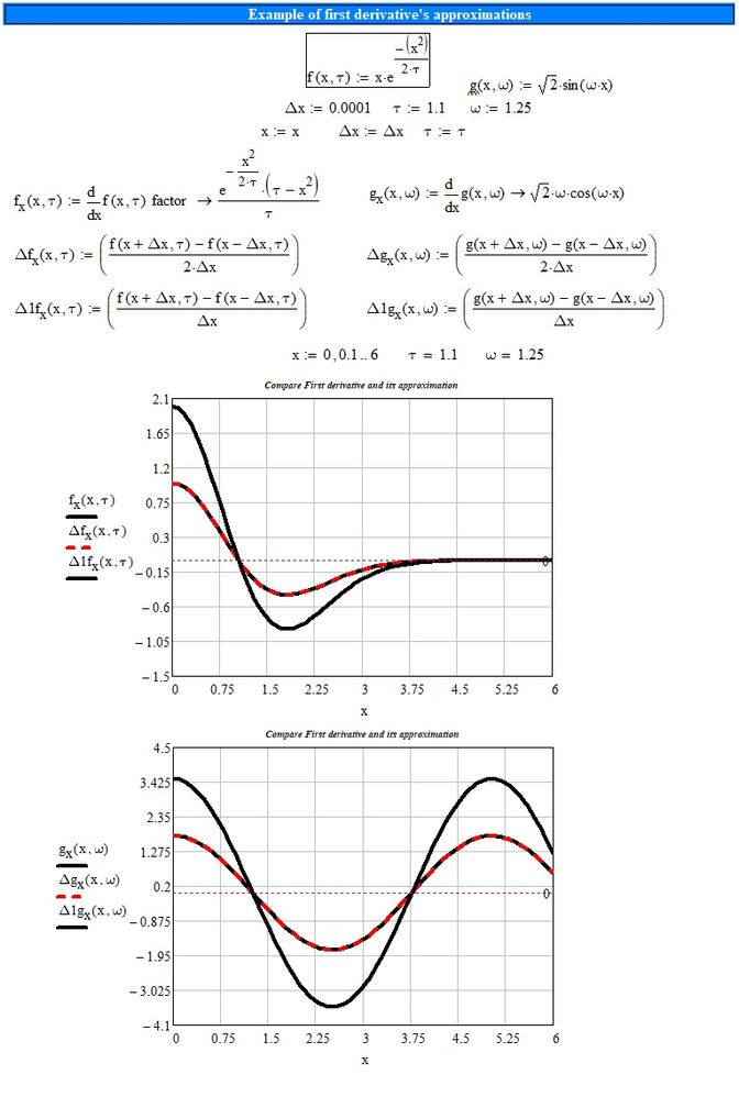
I have not elaborated on the approximations that you have made. However, with regard to the first derivative of a function and its approximation, we must be careful, the following graphs highlight this fact:
- Mark as New
- Bookmark
- Subscribe
- Mute
- Subscribe to RSS Feed
- Permalink
- Notify Moderator
hi there,
thanks for looking over the examples. i'm not sure i follow you. as far as i know the method i used is producing the same results as the built in derivative and second derivative functions. that is what is in the comparison files. however, the built in functions become extremely slow. sometimes you have to use different methods as well. so i think manually doing it is better. i don't see a problem in the files i created. but if you do, please let me know. you can message me here as well. i did have to do one thing different than i normally do, to match mathcad. i had to use a forward point and a backward point. i usually just use backwards points. but i still didn't see any issue.
note; on the comparison files you might want to change the inputs, so you don't have to wait so long for the built in derivatives to complete. i think i have some of those files setup in a way that makes it take really long. my laptop fan goes nuts while it solves those files as well.
thanks,
anthony
- Mark as New
- Bookmark
- Subscribe
- Mute
- Subscribe to RSS Feed
- Permalink
- Notify Moderator
i'm not sure if this is what you are referring to or not. the definitions of forward, backward, and central derivatives. it looks like mathcad is using a central method. i usually use a backward. so i tried to adapt to the central with the provided data. however, technically, you would have to compute points that aren't in the matrix.
https://theailearner.com/2019/05/24/first-order-derivative-kernels-for-edge-detection/
the agreement i was seeing was good though, so i didn't mess with it further.
edit; oh i think i see what you are saying. on your plots, i'm not sure what curve is what. maybe you could change the color of one of the black lines. but i see how the terms cancel and you are left with a divide by 2 that i don't have. i'll look into it more.
edit 2; hmm. adding the divide by 2 introduces a big difference and doesn't agree. so i'm confused now. perhaps message me and we can figure it out. i'm not sure i understand what you were showing. also, not sure why the central difference is different by a factor of 2 to the mathcad derivatives.
edit 3; ahh. what i have is the central difference equation. without the divide by 2. because the delta time is the 2h term. so i think what i have is right.


